Chapter 43: Reasoning Trace Data Engineering: Long-Chain Compression, Implicit Computation, and Supervision Masks¶

Xuan Li; Fengxin Chen

Abstract¶

This chapter uses Latent-Switch-69K as the case study to explain how reasoning-trace data moves from explicit long chain-of-thought to compressible, supervisable, and transferable implicit computation records. The chapter focuses on teacher traces, latent budgets, student sequences, supervision masks, compression boundaries, and quality control, showing that reasoning traces are not ordinary text fields but key data assets connecting reasoning models, post-training, RL data engineering, and reasoning flywheels. It also uses the Latent-Switch MindSpore data pipeline to show how distilled records become training batches consumable by mindspore.dataset.GeneratorDataset.

Keywords¶

reasoning traces; Long-CoT; Latent-Switch-69K; implicit computation; supervision masks; reasoning data engineering

Latent-Switch-69K: Reasoning Trace Compression and Latent Compute Slots¶

Learning Objectives¶

After completing this chapter, readers should be able to:

Understand the engineering constraints of Long-CoT with respect to token cost, explicit process supervision, and reasoning efficiency, and explain why compression is necessary.
Describe the roles of solution intuition, compressed CoT, latent placeholders, and answer masks within a latent-then-explicit sample.
Design mask invariants and consistency checks governing latent budgets, student sequences, and supervision masks.
Evaluate risks in reasoning data compression, including answer consistency, verification sufficiency, compression boundaries, and domain bias.
Transfer the latent-switch concept of separating hidden planning from explicit verification to custom datasets in mathematics, code, and complex instruction-following tasks.

43.1 Opening Problem: Why Does Long-CoT Still Need to Be Compressed¶

Chapters 18 through 20 have already covered the basic forms of Chain-of-Thought data, tool-call traces, and agent interaction data. For reasoning models, long chains of thought carry obvious appeal: the model writes out intermediate steps, allowing trainers to inspect whether it is solving problems along some interpretable path, and making it easier at inference time to detect errors through self-consistency sampling, verifiers, or process reward models. However, once Long-CoT transitions from research examples into training corpora, the problems immediately become engineering problems.

First, long CoT carries a high token cost. Derivations in mathematics, code, and science problems typically dominate the output length, while the actual final answer occupies only a small fraction. If all intermediate reasoning enters training and inference as visible text, the model must spend context window capacity, training memory, and inference time on large amounts of repetitive, unrolled, exploratory, and self-correcting text. Second, long CoT does not naturally equate to high-quality reasoning. Some traces merely decompose simple conclusions into many steps; some contain erroneous branches; and some produce redundant or even inconsistent intermediate explanations while still arriving at a correct final answer. Third, standard SFT has difficulty distinguishing "high-level problem-solving intent that should be internalized by the model" from "verification steps that must be written out explicitly for the user." If the entire CoT is treated as ordinary target tokens, models tend to learn the writing habit of lengthy elaboration rather than a more effective reasoning scheduling strategy.

Latent-Switch-69K emerged against this backdrop. It is neither a simple "shorter CoT dataset" nor a collection of Long-CoT samples summarized and directly used for SFT. It serves LaTER-style latent-then-explicit reasoning systems, while Latent-Switch MindSpore implements the data loading, span materialization, and mask construction pieces as a MindSpore data pipeline: the model first passes through a bounded latent reasoning interval, completing high-level planning and compressed thinking in continuous hidden states, then switches back to visible text and uses a shorter explicit CoT for symbolic verification, before generating the final answer. The data engineering objective therefore shifts: samples must answer not only "what is the answer" but also "which content is appropriate for the hidden planning budget and which content still needs to serve as visible verification supervision."

Figure 43-1 illustrates the corresponding workflow or structure.

Figure 43-1: Latent-Switch-69K distills reasoning traces from Dolci-Think-SFT-32B into solution intuitions, compressed CoT, latent budgets, student sequences, and mask-aligned SFT records.

This chapter builds on Part 5's synthetic data engineering and Part 6's reasoning data engineering. Chapters 15 through 17 discuss how to generate, distill, and quality-check high-quality training samples; Chapter 18 covers the organization of explicit CoT; and Chapters 19 and 20 cover the recording of intermediate states in tool and agent traces. Latent-Switch-69K pushes these threads to a finer level: intermediate reasoning need not always be stored as natural language, and datasets can explicitly reserve slots for hidden computation. Looking ahead, this chapter connects naturally to Chapter 45 on post-training data recipes, Chapter 46 on RL reasoning data engineering, and the reasoning flywheel projects in Part 14 (P06, P10, P12).

43.2 Dataset Overview: Scale, Difficulty, and Domain Composition¶

The final training split of the Latent-Switch-69K dataset contains 69,745 samples. Each retained sample includes a user question, a distilled solution intuition, a shortened explicit CoT, a final answer, latent-step metadata, and masks that determine how different token spans are supervised during training. This structure distinguishes it from ordinary CoT/SFT data: standard SFT records typically require only a prompt and an assistant output, and standard CoT data typically requires only that reasoning and the answer be written inside <think> tags or natural-language paragraphs. Latent-Switch-69K additionally records a budget for hidden planning and renders that budget as latent placeholders in the student sequence.

In terms of difficulty distribution, the dataset does not pursue perfect uniformity. Medium-difficulty samples constitute the majority at 45,650 samples (65.5%); hard samples account for 17,428 (25.0%); and easy samples account for 6,667 (9.5%). This distribution has a clear rationale for latent-switch training. Medium-difficulty questions typically require genuine reasoning rather than templated question-answering, yet they are not so complex as to destabilize the distillation process. Hard samples provide longer, more complex reasoning chains, exposing the model to higher-budget implicit planning scenarios. Easy samples help the model retain the ability to produce short answers and direct verifications, preventing all samples from being cast as long-reasoning tasks.

Table 43-1 summarizes the corresponding comparison and engineering considerations.

Table 43-1: Dataset Overview: Scale, Difficulty, and Domain Composition.

Statistic	Value	Share / Notes
Total examples	69,745	100.0%
Easy	6,667	9.5%
Medium	45,650	65.5%
Hard	17,428	25.0%
Compression ratio mean	0.612	distilled CoT length / original CoT length
Compression ratio median	0.569	The median sample retains approximately 56.9% of the explicit reasoning length
Latent steps mean	41.49	Average number of latent placeholders per sample
Latent steps median	40.00	The median sample has approximately 40 latent steps

In terms of domain composition, Latent-Switch-69K skews heavily toward reasoning-intensive tasks. Mathematics problems account for approximately 37%, code problems for approximately 34%, science-oriented questions for approximately 5%, and the remainder comes primarily from instruction-following and general-knowledge prompts. This proportion is not accidental. The tasks that most benefit from latent-then-explicit reasoning are those that involve "a high-level solution plan but where one does not want to unroll all derivations"; mathematics and code have strong verifiability, clear step structure, and high token costs. Science questions provide conceptual reasoning and multi-condition judgment scenarios, while general instruction and knowledge samples prevent the model from learning only the expression patterns of competition mathematics or code completion.

Figure 43-2 illustrates the corresponding workflow or structure.

Figure 43-2: The final training set contains 69,745 samples; mathematics, code, and precise instruction-following data account for a large share.

From a data engineering perspective, three classes of statistics must be preserved simultaneously. The first is scale statistics, which confirm that the training set is large enough to serve as a dedicated latent reasoning supervision corpus rather than a small collection of prompt templates. The second is difficulty statistics, confirming that data is not stacked randomly but serves curriculum stability and latent budget stability. The third is domain statistics, clarifying that this dataset is best suited for training and evaluating reasoning tasks in mathematics, code, science, and complex instructions, and should not be misread as general-purpose SFT data covering all conversational scenarios.

Latent-Switch-69K retains the following fields: dataset_name, source_dataset, record_id, difficulty, domain, source_cot_length, distilled_cot_length, compression_ratio, solution_intuition_length, n_latent_steps, assistant_cot, assistant_answer, and mask_schema_version. These fields may appear primarily engineering-oriented, but they determine whether one can later explain whether a given training result stems from a shorter CoT, a latent budget adjustment, or a change in domain proportions.

Looking more closely, the fields of Latent-Switch-69K fall into four groups. The first group is provenance fields, which record where a sample came from, which task family the original question belongs to, and whether it originates from mathematics, code, science, or general instruction data. Provenance fields are not decorative; they govern downstream mixing, deduplication, and accountability. For example, when a model improves on code tasks but becomes verbose on open-ended question answering, engineers need to return to the provenance fields to check whether code sample weights are too high or whether instruction-following samples have been compressed too short.

The second group is reasoning content fields, comprising the source reasoning trace, solution intuition, assistant_cot, and assistant_answer. The source trace is the reference prior to distillation and does not necessarily enter the final student sequence; the solution intuition is the high-level plan; the assistant_cot is the compressed explicit verification chain; and assistant_answer is the final answer. These four elements must maintain a traceable relationship. Ideally, an auditor can start from a single training sample and trace back: which information from the original long CoT was distilled into the intuition, which necessary derivations remain in the compressed CoT, and whether the answer is consistent with the verifiable target of the original question.

The third group is length and budget fields, including source CoT length, distilled CoT length, intuition length, compression ratio, and n_latent_steps. These fields directly serve cost control and budget diagnostics. If the average compression ratio of a data version suddenly drops to 0.3, the token cost appears lower, but this may indicate that the explicit verification chain has been compressed too short. If the mean n_latent_steps suddenly rises, the effective sequence length during training and the hidden computation cost at inference both increase. Without these length fields, teams cannot make quantitative judgments between "efficiency gains" and "supervision loss."

The fourth group is supervision fields, including prompt_mask, latent_internal_mask, latent_boundary_mask, cot_mask, answer_mask, and teacher_kl_mask. These masks determine how the same token sequence is interpreted during training. Ordinary dataset schemas typically care only about whether text fields are present; Latent-Switch-69K must also treat masks as data assets. The reason is straightforward: the same span of text, given different masks, corresponds to a different training objective. A latent placeholder fitted with CE becomes an ordinary token; masked and replaced by a recurrent latent state, it becomes a hidden computation slot.

43.3 Distillation and Record Formation: From Teacher Trace to Compressed Reasoning Record¶

The starting point for constructing Latent-Switch-69K is reasoning traces sampled from Dolci-Think-SFT-32B. These original traces, understood as source reasoning traces, contain the question, one or more assistant outputs, a possible ground truth or extractable answer, and source and metadata. The construction process does not directly filter for short answers; instead, it first decomposes long traces into two complementary objectives: a high-level problem-solving intent and a shorter explicit verification chain.

The following pedagogical example shows the simplest way to extract source traces: load Dolci-Think-SFT-32B from Hugging Face, shuffle it with a fixed random seed, select a batch of records, and normalize the conversations into the minimum fields required for subsequent distillation. Within the responsibility boundary of Latent-Switch MindSpore, this step and the subsequent teacher API call are upstream data preparation; the MindSpore repository consumes already-distilled rows containing stage1.correct_insight, stage2.distilled_cot, and stage2.answer.

Listing 43-1 provides a Python implementation excerpt.

from datasets import load_dataset


def first_message(messages, role):
    return next(
        (item["content"] for item in messages if item.get("role") == role),
        "",
    )


def last_message(messages, role):
    return next(
        (item["content"] for item in reversed(messages) if item.get("role") == role),
        "",
    )


dataset = load_dataset("allenai/Dolci-Think-SFT-32B", split="train")
sample_size = min(2000, len(dataset))
sampled = dataset.shuffle(seed=42).select(range(sample_size))

source_traces = []
for row in sampled:
    messages = row.get("messages", [])
    source_traces.append(
        {
            "record_id": row.get("id"),
            "source_dataset": row.get("source", row.get("dataset", "unknown")),
            "problem": first_message(messages, "user"),
            "source_cot": last_message(messages, "assistant"),
        }
    )

Listing 43-1: Python implementation excerpt.

The first stage is extracting the solution intuition. The data construction prompt asks the teacher to extract only key insights—neither writing a short CoT nor directly providing the final answer. This field should describe "the high-level plan for solving this problem," for example which equations to set up, which state space to enumerate, which data structure to use for a coding problem, or which causal relationship to isolate for a science question. Its granularity sits between a label and a full derivation: more specific than a domain label, yet more compressed than step-by-step reasoning. The core value of this approach is extracting the planning signal from Long-CoT that can be internalized, providing the basis for the subsequent latent budget.

The second stage is generating a compressed explicit CoT. The teacher continues solving the problem conditioned on the original question and the solution intuition, producing a shorter reasoning process and a final answer. Because the teacher already has the high-level plan, it does not need to re-expand the full exploration process or repeat invalid branches from the original trace. Each retained sample therefore contains four main components: problem, intuition, compressed CoT, and final answer. Unlike ordinary summarization, the goal of the compressed CoT is not to "shorten the original text" but to retain sufficient visible verification paths so that the model, after latent reasoning, can still complete symbolic checks using text.

The following minimal implementation connects the two stages through an OpenAI-compatible API. The first stage requests only a JSON-formatted correct_insight; the second stage continues from the problem and that intuition, recording the hidden reasoning returned by the API as distilled_cot and the visible content as the final answer. The API key, endpoint, and teacher model are all read from environment variables.

Listing 43-2 provides a Python implementation excerpt.

import asyncio
import json
import os

from openai import AsyncOpenAI


client_kwargs = {"api_key": os.environ["OPENAI_API_KEY"]}
if os.getenv("OPENAI_BASE_URL"):
    client_kwargs["base_url"] = os.environ["OPENAI_BASE_URL"]

client = AsyncOpenAI(**client_kwargs)
teacher_model = os.environ["TEACHER_MODEL"]


async def call_teacher(system_prompt, user_prompt):
    response = await client.chat.completions.create(
        model=teacher_model,
        messages=[
            {"role": "system", "content": system_prompt},
            {"role": "user", "content": user_prompt},
        ],
        extra_body={"thinking": {"type": "enabled"}},
    )
    message = response.choices[0].message
    reasoning = getattr(message, "reasoning_content", None)
    content = message.content or ""

    # Some compatible APIs place reasoning inside the visible content.
    if not reasoning and "<think>" in content and "</think>" in content:
        reasoning, content = content.split("<think>", 1)[1].split("</think>", 1)
    return (reasoning or "").strip(), content.strip()


async def distill_one(problem, source_cot):
    _, insight_json = await call_teacher(
        "Return valid JSON with one field named correct_insight. "
        "Give only the high-level solution plan, without the final answer "
        "or a complete chain of thought.",
        f"Problem:\n{problem}\n\nReference reasoning:\n{source_cot}",
    )
    intuition = json.loads(insight_json)["correct_insight"]

    distilled_cot, answer = await call_teacher(
        "Continue from the supplied solution intuition. Keep the reasoning "
        "compact, verify the key steps, and give the final answer.",
        f"Problem:\n{problem}\n\nSolution intuition:\n{intuition}",
    )
    return {
        "problem": problem,
        "solution_intuition": intuition,
        "distilled_cot": distilled_cot,
        "answer": answer,
    }


record = asyncio.run(
    distill_one(source_traces[0]["problem"], source_traces[0]["source_cot"])
)

Listing 43-2: Python implementation excerpt.

Figure 43-3 illustrates the corresponding workflow or structure.

Figure 43-3: The extensive visible reasoning in the source trace is split into two types of signal: solution intuition is used to estimate the latent budget, and the compressed CoT is used for explicit verification and answer supervision.

The compression ratio is defined as:

\[ \text{compression ratio} = \frac{\text{distilled CoT length}}{\text{original CoT length}}. \]

The mean compression ratio across the final corpus is 0.612 and the median is 0.569. This indicates that the distilled visible CoT typically retains approximately 57% to 61% of the original reasoning length. This figure should not be interpreted as "forty percent of reasoning information has been deleted." A more accurate reading is: some details have been compressed into the high-level plan represented by the solution intuition and further mapped onto the latent placeholder budget, while the necessary derivations still retained inside <think> serve for explicit verification and to supervise the model's visible reasoning style.

Figure 43-4 illustrates the corresponding workflow or structure.

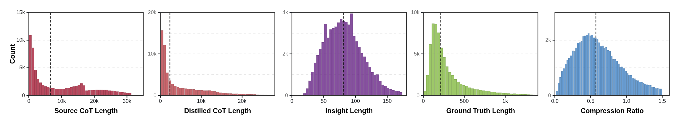
Figure 43-4: This figure shows the distributions of source CoT length, distilled CoT length, intuition length, ground truth length, and compression ratio.

Sample retention criteria should revolve around three questions. First, does the source trace have a sufficiently reliable final answer? If the original answer cannot be extracted, is clearly inconsistent with the ground truth, or cannot be stably reproduced by the teacher, the sample is not suitable for the final set. Second, does the solution intuition express only the high-level plan? If the intuition directly discloses the answer or is written as a complete CoT, it is no longer appropriate as a proxy for the latent budget. Third, does the compressed CoT still connect the question to the answer? If compressed too aggressively, the explicit reasoning degenerates into a few disconnected sentences; the model may imitate the answer but fails to learn the boundary between switching from implicit planning to explicit verification.

This distillation process offers an important lesson for data engineering teams: reasoning data compression cannot focus solely on token counts. More reliable compression must simultaneously check intent preservation, answer consistency, and verification sufficiency—that is, compressed samples must retain the problem-solving intent, preserve sufficient visible verification paths, and maintain consistency in the final answer.

Mapping this pipeline to an engineering system, it can be decomposed into six auditable stages. Stage one is source trace extraction: unifying prompts, assistant outputs, ground truth, dataset source, and metadata from Dolci-Think-SFT-32B into internal records. The most important task at this stage is to preserve the original context rather than rewriting it prematurely, because if teacher outputs turn out to be anomalous, engineers need to return to the source trace to determine whether the error originated in the original trace, the prompt template, or the answer extraction step.

Stage two is high-level intuition distillation. The prompt explicitly instructs the teacher to return JSON and constrains correct_insight to describe only a coarse-grained plan—without providing the final answer and without writing a complete CoT. This constraint is critical because the role of the intuition is not to train the model to "repeat this text," but to estimate how much hidden planning space to allocate to the model. If the intuition already contains detailed derivations, the latent budget shifts from "compressing planning complexity" to "copying the length of an invisible CoT," which undermines the clarity of the data design.

Stage three is compact explicit CoT generation. The teacher generates a shorter reasoning chain conditioned on the original question and the intuition, in effect reorganizing the publicly verifiable portion of the source trace. Two extremes must be avoided: on one end, a CoT that is still very long with almost no compression; on the other end, only a conclusion remains with no verification. Well-formed samples typically retain key equations, key branches, key code invariants, or the rationale for a final choice, while removing repetitive scaffolding, self-doubt, and futile explorations.

Stage four is answer validation. For mathematics problems, one can check whether the extracted answer is consistent with the ground truth; for multiple-choice problems, one can check the option format; for code problems, one should attempt unit tests or static rule checks; and for open-ended questions, at minimum a teacher consistency check or sampled human review is required. Latent-switch training depends on answer consistency more heavily than ordinary summarization tasks, because answer tokens are the primary supervision location for correctness, and incorrect answers will be learned by the model together with the latent budget and explicit CoT.

Stage five is sequence rendering. The system renders the problem, latent placeholders, compressed CoT, and answer into a chat-style student sequence. This stage requires a tokenizer contract: <latent_think>, </latent_think>, <think>, and </think> must be recognized stably and must not be split into unpredictable fragments by different tokenizers or different special-token registration methods. Otherwise, span detection and mask construction will both be unreliable.

Stage six is mask materialization. The data loader re-locates boundaries based on token IDs and constructs labels, loss weights, and various masks. This stage should not rely solely on character offsets in the raw string, because changing the tokenizer will invalidate character offsets. A more robust approach is to construct spans based on the positions of special tokens in the token ID sequence, and to validate for each sample that boundary token counts, ordering, answer span, and teacher-reference span are all valid.

43.4 Latent Budget and Student Sequence: How Samples Are Rendered¶

One of the key fields in Latent-Switch-69K is n_latent_steps. It determines how many latent placeholders are placed between <latent_think> and </latent_think> in the student sequence. The basic heuristic adopted in the paper and code is: if the retained solution intuition contains \(L\) tokens, the latent budget is approximately \(L/2\), clipped by a maximum latent length and tokenizer constraints. In the final data, the mean latent step count is 41.49 and the median is 40.00.

This budget rule carries two implications. First, latent steps are not arbitrary padding; they are correlated with the compressed high-level reasoning content. A longer intuition suggests that the high-level planning for this problem may be more complex, and the model therefore requires more hidden computation slots. Second, more latent steps are not unconditionally better. An excessively long latent interval increases training and inference costs and may allow the model's hidden state to drift. In Latent-Switch-69K, the final samples concentrate around roughly 40 latent steps; the MindSpore data pipeline constrains this budget through latent_min, latent_max, and a hard 256-step ceiling in SFTBuildConfig.

In the student sequence, a sample can be abstractly written as:

\[ \mathrm{LATENT}_{1:m} \;\rightarrow\; \mathrm{THINK}_{1:n} \;\rightarrow\; \mathrm{ANSWER}_{1:r} \;\rightarrow\; \mathrm{EOS}. \]

Here \((l_1,\dots,l_m)\) are latent placeholder positions, \((t_1,\dots,t_n)\) are the distilled explicit CoT tokens, and \((a_1,\dots,a_r)\) are the final answer tokens. In the code implementation, latent placeholders can be filled with repeated latent_pad_token entries; however, during training these positions are not treated as ordinary language targets. In the model's forward pass, the input embeddings at placeholder positions are replaced by recurrent latent states produced by a latent projector. In other words, these positions have token boundaries and a defined length in the sequence, but they are semantically hidden computation slots.

The example below follows the real build_sft_record call pattern in Latent-Switch MindSpore records.py. The upstream distilled result enters through stage1 and stage2, while SFTBuildConfig controls compression-ratio filtering, latent budget, loss weights, and the placeholder token. validate_tokenizer_contract in tokens.py first checks that <latent_think>, </latent_think>, <think>, </think>, <|im_start|>, <|im_end|>, and <|endoftext|> are encoded stably.

Listing 43-3 provides a Python implementation excerpt.

import os

from transformers import AutoTokenizer

from latent_switch_mindspore.records import SFTBuildConfig, build_sft_record
from latent_switch_mindspore.tokens import validate_tokenizer_contract


tokenizer = AutoTokenizer.from_pretrained(os.environ["STUDENT_TOKENIZER"])
validate_tokenizer_contract(tokenizer)

distilled_row = {
    "uid": record.get("record_id", "demo-row"),
    "question": record["problem"],
    "stage1": {"correct_insight": record["solution_intuition"]},
    "stage2": {
        "distilled_cot": record["distilled_cot"],
        "answer": record["answer"],
        "validation": {"is_correct": True},
    },
    "token_stats": {"compression_ratio_vs_primary_output": 0.612},
}

config = SFTBuildConfig(
    latent_min=1,
    latent_max=128,
    latent_pad_token="<|endoftext|>",
    cot_loss_weight=0.0,
    answer_loss_weight=1.0,
)
sft_record, reason = build_sft_record(distilled_row, tokenizer, config)
if reason != "ok":
    raise ValueError(f"sample filtered during SFT build: {reason}")

Listing 43-3: Python implementation excerpt.

Production preprocessing additionally filters samples according to compression ratio and field completeness and records the loss weights for the CoT and answer. More importantly, the rendered record must still be passed to materialize_sample or LatentSwitchSFTSource in dataset.py to relocate special-token spans and construct supervision masks. Concatenating this string alone does not make the sample safe for training.

If MindSpore is installed in the runtime, the constructed JSONL can be wrapped directly as a mindspore.dataset.GeneratorDataset. The minimal loading example below shows the training-side columns such as input_ids, labels, teacher_kl_mask, and latent_positions.

Listing 43-4 provides a Python implementation excerpt.

import os

from transformers import AutoTokenizer

from latent_switch_mindspore import create_mindspore_dataset


tokenizer = AutoTokenizer.from_pretrained(os.environ["STUDENT_TOKENIZER"], use_fast=True)
dataset = create_mindspore_dataset(
    "data/sft_train.jsonl",
    tokenizer=tokenizer,
    batch_size=2,
    max_length=4096,
    shuffle=False,
)

for batch in dataset.create_dict_iterator(output_numpy=True, num_epochs=1):
    print(batch["input_ids"].shape)
    print(batch["teacher_kl_mask"].shape)
    break

Listing 43-4: Python implementation excerpt.

Below is a pedagogical, simplified sample sequence. It is intended only to illustrate the schema and mask relationships and is not an actual training sample from the dataset.

Listing 43-5 provides a latent-reasoning trace sample.

<|im_start|>user
Target Question:
A sequence satisfies a_1 = 2, a_{n+1} = 3a_n + 1. Find a_4.
<|im_end|>
<|im_start|>assistant
<latent_think>
<|endoftext|><|endoftext|><|endoftext|><|endoftext|>
</latent_think>
<think>
Apply the recurrence relation step by step. Derive a_2 from a_1, then obtain a_3 and a_4.
a_2 = 3 * 2 + 1 = 7;
a_3 = 3 * 7 + 1 = 22;
a_4 = 3 * 22 + 1 = 67.
</think>
The final answer is 67.
<|im_end|>

Listing 43-5: Latent-reasoning trace sample.

In this example, <latent_think> and </latent_think> are structural boundaries; the four <|endoftext|> tokens in between are merely placeholders, and their count in real samples is determined by n_latent_steps; the region from <think> to </think> is the visible compressed CoT; and the following text is the answer. For training purposes, what matters is not whether this text looks like natural conversation, but whether each token span can be stably located. build_spans in Latent-Switch MindSpore checks that a sample contains exactly one <latent_think>, one </latent_think>, one <think>, and one </think>, and verifies that they satisfy:

Listing 43-6 provides a latent-boundary ordering constraint example.

assistant_content_start <= latent_start < latent_end < think_start < think_end

Listing 43-6: Latent-boundary ordering constraint example.

This ordering constraint is critical. If a boundary token is missing, duplicated, or out of order, masks will be misaligned: latent placeholders may be mistakenly treated as ordinary answer tokens, or the answer span may be truncated. For ordinary SFT data, a boundary error may be merely a formatting issue; for latent-switch data, a boundary misalignment directly changes the training objective.

In a production data warehouse, student sequences should not be stored solely as long strings. A more robust approach is to save both structured fields and rendered text in parallel. Structured fields include messages, assistant_cot, assistant_answer, n_latent_steps, latent_pad_token, and state_align_reference_messages; rendered text is used for quick inspection and compatibility with standard training frameworks. LatentSwitchSFTSource uses structured fields to construct token IDs, and materialize_sample then creates labels, loss weights, and the mask columns. This design reflects an empirical lesson: latent special-token boundaries are too important to depend entirely on pre-concatenated text.

latent_pad_token also deserves separate attention. Its role in the sequence is to occupy space rather than carry semantic content. If the tokenizer has already registered this token, the data loader can directly repeat its ID; if not, the string must be repeated and then re-encoded, introducing length uncertainty. For an ordinary padding token this discrepancy may be acceptable; for the latent budget, it changes the actual token count \(m\) and consequently the number of steps in the hidden rollout. Datasets should therefore explicitly document the tokenizer version, special-token registration method, and the semantics of the latent pad token at release time.

The teacher-reference conversation is another sequence that is easy to overlook. It is not a copy of the student sequence; rather, it is a reference conversation constructed by omitting latent placeholders. The teacher input contains the original question and the solution intuition, and the assistant continuation is the compressed CoT and the answer. This design focuses teacher KL supervision on visible reasoning quality and answer distribution rather than requiring the teacher to understand the student's internal latent slots. In other words, the student sequence trains the latent-then-explicit format, while the teacher reference provides a distributional reference for the explicit verification portion; the two serve different supervision objectives.

43.5 Supervision Masks: Which Tokens Contribute to the Loss¶

The supervision design of Latent-Switch-69K can be summarized in one sentence: prompt tokens and latent interior placeholders do not participate in ordinary token-level CE; structural boundaries, explicit CoT, answers, and end tokens participate in targeted supervision; and teacher KL applies only to selected explicit CoT and answer positions.

In the code implementation, each sample generates multiple masks: prompt_mask, latent_internal_mask, latent_boundary_mask, cot_mask, answer_mask, and teacher_kl_mask. These masks are not merely for visualization convenience; they directly determine the positions where different objectives take effect. Ordinary labels are initialized from student token IDs, and then positions within the prompt span and latent interior span are set to -100, indicating that they are ignored by cross-entropy.

The CE label rule can be expressed in simplified form as:

\[ y_i = \begin{cases} -100, & i \in \mathcal{S}_{\mathrm{prompt}} \cup \mathcal{S}_{\mathrm{latent\_inner}}, \\ x_i, & \text{otherwise}. \end{cases} \]

Here \(\mathcal{S}_{\mathrm{prompt}}\) denotes positions in the user prompt and the context preceding the assistant prefix, and \(\mathcal{S}_{\mathrm{latent\_inner}}\) denotes the interior placeholder positions between <latent_think> and </latent_think>. Tokens set to -100 are not directly fitted by ordinary CE. This avoids an erroneous objective: requiring the model to predict a specific fixed text token at latent interior positions. For latent-switch data, the value of latent interior positions lies not in outputting <|endoftext|> tokens but in reserving slots for hidden state updates; the MindSpore data pipeline writes these positions explicitly into latent_internal_mask, latent_positions, and latent_slot_mask.

Figure 43-5 illustrates the corresponding workflow or structure.

Figure 43-5: Prompt and latent interior tokens are masked from ordinary CE; latent boundaries, explicit CoT, answers, and end tokens are controlled by different weights and masks.

latent_boundary_mask marks the two boundary positions <latent_think> and </latent_think>. The boundary tokens themselves still require supervision, because the model must learn when to enter the latent interval and when to exit it. Without supervision of boundaries, the model may fail to transition stably to <think>, or may generate incomplete structure at inference time.

cot_mask covers the span from <think> to the position before answer_start. In the paper's training objective, interior explicit CoT tokens may use a different weight—for example, applying a factor \(\lambda_{CoT}\) to reduce the dominance of explicit reasoning over the total CE loss. This is consistent with the dataset's goals: the explicit CoT remains important because it carries verification and interpretable output, but training should not degenerate into "the more it resembles a long CoT, the better." The model must primarily learn structural boundaries and final-answer behavior.

answer_mask covers the answer span between </think> and <|im_end|>. Answer tokens should generally receive strong supervision, because the final answer is the primary site of task correctness. For mathematics problems it may be a boxed answer; for multiple-choice problems it may be A, B, C, or D; for code problems it may be a function implementation. Regardless of how the latent interval is designed, answer consistency must be strictly maintained.

teacher_kl_mask is used for teacher-distribution supervision. Each sample also generates a teacher-reference conversation: it contains no student latent placeholders; instead, it merges the original question and the distilled solution intuition as teacher input and provides a distributional reference at the shortened <think> ... </think> and answer positions. The benefit is that the teacher does not need to simulate continuous latent placeholders; it supervises only the token distribution quality of explicit reasoning and the answer.

Table 43-2 summarizes the corresponding comparison and engineering considerations.

Table 43-2: Supervision Masks: Which Tokens Contribute to the Loss.

Span	Example tokens	CE label	Primary mask	Engineering significance
Prompt and assistant prefix	user question `<\\|im_start\\|>assistant`	`-100`	`prompt_mask`	Serves as conditioning, not as output target
Latent start boundary	`<latent_think>`	supervised	`latent_boundary_mask`	Model learns to enter latent reasoning
Latent interior slots	`l_1 ... l_m`	`-100`	`latent_internal_mask`	Hidden computation slots; placeholder text is not fitted
Latent end boundary	`</latent_think>`	supervised	`latent_boundary_mask`	Model learns to stop latent reasoning
Explicit reasoning	`<think> ... </think>`	weighted supervised	`cot_mask`, `teacher_kl_mask`	Visible verification chain; weight may be reduced
Final answer	answer tokens	supervised	`answer_mask`, `teacher_kl_mask`	Core supervision for task correctness
End token `<\\|im_end\\|>`	supervised	end-token weight	`answer_mask`	Ensures chat format closure

This mask design explains why Latent-Switch-69K cannot be arbitrarily re-encoded by ordinary data loaders. Ordinary chat data loaders typically care only about the boundary between prompt and response, whereas a latent-switch data loader must know the precise positions of latent_start, latent_end, think_start, think_end, answer_start, and im_end. Any inconsistency in special-token registration or any string re-encoding that shifts boundary token positions will corrupt the masks.

More precisely, the masks also decouple different training objectives. The CE objective trains the model to output structural boundaries, explicit reasoning, and answers; the latent internal mask protects hidden computation slots, preventing the model from learning them as ordinary text; the teacher KL objective brings explicit CoT and answers closer to the teacher's distribution; and halt or boundary-related supervision helps the model terminate latent reasoning at appropriate positions.

For data engineers, the most practical check is not to re-derive the loss function but to confirm that each sample's masks satisfy several invariants. First, all labels in the prompt span should be -100. Second, all labels in the latent interior span should be -100, but latent boundary tokens should not be treated as ordinary prompt masks. Third, cot_mask should cover the positions associated with <think> through </think>, and answer_start must come after think_end. Fourth, answer_mask should not include <|im_end|>, since the end token can be supervised independently. Fifth, the teacher KL mask should not cover the latent interior, because the teacher reference itself contains no such placeholders.

These invariants should be checked at both the data construction stage and the training data-loading stage. Construction-stage checks prevent bad samples from entering the database; loading-stage checks catch new problems introduced by tokenizer changes, max_length settings, truncation strategies, or configuration updates. Truncation by max_length is a particular concern: once the answer span is truncated, the sample contains only structure and reasoning with no final-answer supervision. The code therefore reconstructs spans after truncation and checks that answer_start is still less than im_end.

Another detail worth noting is the weight applied to explicit CoT. Latent-Switch-69K does not aim to delete explicit reasoning but to reduce dependence on complete long CoT. If CoT weight is too high, the model will tend to direct its capacity toward reproducing visible reasoning text; if too low, the model may learn only structure and answers while the explicit verification chain weakens. On the data side, at minimum a configurable cot_loss_weight or equivalent field should be retained, enabling trainers to adjust the balance between "visible verification" and "final answer" for different tasks.

43.6 Quality Control: Five Categories of Risk in Compression, Boundaries, and Bias¶

Quality control for Latent-Switch-69K is not merely about filtering dirty text. Because the dataset simultaneously contains compressed reasoning, latent budgets, and multiple masks, risks are distributed across multiple layers.

Table 43-3 summarizes the corresponding comparison and engineering considerations.

Table 43-3: Quality Control: Five Categories of Risk in Compression, Boundaries, and Bias.

Risk type	Typical symptom	Impact	Remediation
Over-compression	Compressed CoT contains only a conclusion with no visible verification chain	Model fails to learn the transition from latent planning to explicit verification	Add verification sufficiency checks; reject samples with missing steps
Reasoning discontinuity	Solution intuition and compressed CoT follow different solution paths	The high-level plan associated with the latent budget cannot support the subsequent CoT	Check intuition–CoT entailment; require teacher to regenerate
Answer inconsistency	Source, teacher continuation, and final answer are inconsistent	Training objective conflicts at answer positions	Cross-check with ground truth, a verifier, or answer extraction rules
Boundary misalignment	`<latent_think>` or `<think>` tokens are missing, duplicated, or out of order	Mask misalignment causes latent placeholders to be supervised incorrectly	Perform span validation before data ingestion; quarantine invalid samples
Domain bias	Math and code are over-represented; general instruction coverage is insufficient	Model style narrows when transferred to non-reasoning tasks	Record domain mix; adjust sampling weights according to training objectives
Abnormal latent budget	`n_latent_steps` is 0, excessively large, or mismatched with intuition length	Implicit planning budget is distorted; inference cost becomes uncontrollable	Set upper and lower bounds on budget; monitor mean, median, and tail
Teacher KL misalignment	KL mask does not align with teacher reference tokens	Teacher-distribution supervision acts on incorrect positions	Retain teacher span validation; record top-k distribution version

The first risk is over-compression. A mean compression ratio of 0.612 and median of 0.569 confirm that the corpus significantly shortens visible CoT, but it would be wrong to treat a lower compression ratio as always better. If a sample compresses 1,000 reasoning tokens down to 50 tokens but loses key equations, state transitions, or code invariants, it saves tokens while undermining supervision quality. A more robust metric is compositional: the compressed length is shorter, the answer remains consistent, and the visible reasoning can still explain the final answer.

The second risk is reasoning discontinuity. The solution intuition is the source of the latent budget; if the intuition describes one solution path while the compressed CoT actually follows a different one, the model receives inconsistent signals. For example, the intuition might say "use dynamic programming" while the compressed CoT uses a greedy proof, or the intuition might say "first establish equations" while the subsequent text directly enumerates cases. In such situations the placeholder count may still be reasonable, but the high-level plan it represents is mismatched. The data pipeline must check semantic consistency between intuition and CoT.

The third risk is answer inconsistency. One of the most common problems in reasoning data is that intermediate chains appear reasonable but the final answer differs from the ground truth. For Latent-Switch-69K, answer inconsistency is more serious, because the teacher reference, the student sequence, and the answer_mask are all constructed around the final answer. If an incorrect answer enters training, the model not only learns an incorrect conclusion but may also learn an incorrect latent-to-explicit switching pattern. Mathematics and multiple-choice problems can use rule-based verifiers or answer extractors; code problems can use unit tests; open-ended questions require at minimum a teacher consistency check or sampled human review.

The fourth risk is boundary and mask misalignment. <latent_think>, </latent_think>, <think>, and </think> are structural tokens, not ordinary text decorations. The data loader checks their counts and order and computes spans accordingly. If a sample has an extra </think>, ordinary rendering may still display correctly, but training masks will be misaligned. Quality control should place span validation before data ingestion rather than waiting for training errors.

The fifth risk is domain bias. With mathematics at approximately 37%, code at approximately 34%, and science at approximately 5%, Latent-Switch-69K is well suited for reasoning-heavy training but is not a complete replacement for general-purpose assistant corpora. When mixing it with ordinary SFT data, the training objective should be stated explicitly: whether the goal is to strengthen mathematical and code reasoning, compress visible CoT, or improve response efficiency across all user queries. Different objectives correspond to different sampling weights and evaluation sets.

Quality control must also retain audit information. Each data version should produce at minimum four reports: a length and compression ratio report, a difficulty/domain distribution report, a span and mask validation report, and an answer consistency and failure sample report. For latent reasoning data, having only the final Parquet or JSONL file is insufficient; without these reports it is very difficult after training to determine whether model changes stem from improved data quality or from unintended distribution drift.

To make these reports genuinely useful, a pre-release acceptance checklist should be established for Latent-Switch-69K. At the length level, check the distributions of source CoT, distilled CoT, intuition, answer, and total sequence, with particular attention to overly short and overly long samples. Short samples may provide insufficient supervision; long samples may be truncated frequently during training. At the compression level, check the mean, median, percentiles, and extreme values of the compression ratio, confirming that no single source dataset is causing anomalies.

At the structural level, check each sample individually for the count and order of the four boundary tokens. Any absence, duplication, nesting, or ordering error should trigger immediate quarantine. At the mask level, sample-render token spans and display the prompt, latent interior, latent boundary, CoT, answer, and im_end regions in distinct colors to confirm that manual interpretation agrees with the programmatic mask. For any new data source, it is advisable to manually review at least a few dozen samples, especially long mathematical proofs, code functions, multiple-choice questions, and open-ended answers.

At the semantic level, check whether intuition contains the final answer, whether the compressed CoT can support the answer, and whether the answer is consistent with the ground truth or a verifier. For code tasks, one should where possible distinguish between "the reasoning explanation is conceptually correct" and "the final code executes correctly." For mathematics tasks, one should distinguish between "the final numerical value is correct" and "the derivation chain is verifiable." Since the goal of latent-switch data is high-level planning plus explicit verification, neither level can be entirely abandoned.

At the distribution level, check the joint distribution of difficulty, domain, source dataset, language, answer format, and token length. Individual fields may each appear normal, but combinations may reveal bias. For example, hard samples may come almost entirely from mathematics, code samples may almost all use one particular Python template, and instruction samples may have a significantly lower compression ratio than mathematics samples. These biases need not all be eliminated, but they must be documented because they will influence downstream training and evaluation.

At the versioning level, each release should include a data version number, build script version, teacher model version, tokenizer version, special-token contract, filtering rules, and statistical reports. The auditability of a dataset like Latent-Switch-69K derives from the combination of text, structure, and configuration. If only the final text is preserved, it will be very difficult years later to explain why a given sample has 38 latent steps, why a particular CoT was down-weighted, or why certain teacher KL positions were skipped.

43.7 Cross-Chapter Links: From Reasoning Data to the Reasoning Flywheel¶

Placing Latent-Switch-69K back within the book's overall structure, its value lies not in introducing an isolated dataset but in demonstrating a new interface for reasoning data.

With respect to Part 5, it extends the core ideas of synthetic and distillation data. Chapter 15 emphasizes designing samples from a task definition for data synthesis; Chapter 16 discusses how distillation transfers strong model behavior into training corpora; Chapter 17 discusses quality assessment and filtering. Latent-Switch-69K concretizes these principles: extracting high-level solution intuitions from teacher traces, preserving explicit verification with compressed CoT, and using masks to assign different supervision objectives to different token spans.

With respect to Part 6, it represents the next step in CoT data engineering. CoT samples in Chapter 18 typically supervise the reasoning process directly as text; tool-use data in Chapter 19 emphasizes actions, observations, and outcomes; agent data in Chapter 20 emphasizes states and trajectories. Latent-Switch-69K shows that reasoning states can also be partially stored in invisible latent slots. It does not abandon interpretability; rather, it compresses visible explanation to the necessary verification chain and migrates exploratory planning into the hidden computation interval.

With respect to Part 13, it serves as a prerequisite template for post-training and RL reasoning data recipes. Chapter 45 discusses the data hierarchy for SFT, preference alignment, and online continuous optimization; Chapter 46 discusses RL reasoning, verifiers, candidate groups, and reward signals. Latent-Switch-69K introduces structured reasoning budgets and mask schemas at the SFT stage, enabling subsequent RL stages to continue optimizing around "whether the latent budget is appropriate," "whether explicit verification is sufficient," and "whether the answer is verifiable."

With respect to Part 14 projects, it can interface with P06, P10, and P12 respectively. P06's PRM data focuses on scoring individual process steps; Latent-Switch-69K provides compressed explicit reasoning and answer spans, suitable for further extracting scorable verification steps. P10's LLM data flywheel focuses on online feedback and continuous iteration; latent-switch data can serve as a candidate data asset for reducing inference token costs. P12's R1 reasoning flywheel focuses on multi-sample generation, verifiers, and rejection sampling; Latent-Switch-69K provides a cold-start approach: first use distillation data to teach the model how to switch between latent planning and explicit verification, then use verifiers and RL data to further adjust the budget and answer correctness.

Finally, the engineering conclusions of this chapter can be compressed into four points.

Latent reasoning data is not a short version of ordinary CoT data. It must record the relationships among the hidden planning budget, the explicit verification chain, and the final answer.
<latent_think> and <think> are structurally distinct intervals with different semantics. The former provides implicit computation slots; the latter provides visible reasoning supervision.
Masks are part of the data schema, not an implementation detail appended to training code. Prompt, latent interior, boundary, CoT, answer, and teacher-KL positions must all be stably recoverable at data construction time.
The goal of data compression is not to delete reasoning but to redistribute high-level intent, hidden computation, and explicit verification into more appropriate channels.

If a team reuses only the text output of Latent-Switch-69K while ignoring n_latent_steps, latent boundaries, and supervision masks, the result is merely a shorter CoT SFT dataset. Only by managing compression ratio, latent placeholders, student sequences, and masks as a unified data engineering artifact does the dataset fully embody the design principles of latent-then-explicit reasoning.

43.8 Reuse Recommendations: Transferring the Latent-Switch Approach to Custom Data¶

If a team wishes to apply the ideas behind Latent-Switch-69K to their own mathematical, code, or business reasoning data, the recommended first step is not to modify the model architecture. A more prudent path is to construct the data schema first. The team can start by extracting a small batch of high-quality questions from existing Long-CoT samples, generating solution intuitions manually or with a teacher model, and then generating compressed CoT and final answers. Next, assign a conservative latent budget based on intuition length—for instance, choosing one or two versions from \(L/3\), \(L/2\), and a fixed 32 steps for comparison. The value of this approach is that the team can first verify whether data can be stably rendered, whether masks are correct, and whether answers are consistent, without immediately committing to expensive training runs.

The second step is to establish a small-scale acceptance set. This set need not be large, but it should cover short problems, long problems, mathematics, code, multiple-choice questions, open-ended questions, and format-constrained prompts. Each sample should be able to answer three questions: does the high-level intuition adequately express the solution plan, does the compressed CoT sufficiently support the answer, and does the latent step count roughly match the problem complexity? If these three criteria frequently fail during manual review, the problem lies not in the training algorithm but in the data construction rules not yet being stable.

The third step is to manage latent-switch data and ordinary SFT data separately. Ordinary SFT data can record only prompt and response; latent-switch data must record structured fields, special-token contracts, mask schemas, and build versions. When mixing for joint training, the sampling weight and intended purpose of each data type should be clearly stated in the manifest. Otherwise, when the model exhibits shortened responses, weaker reasoning explanations, or unstable format boundaries, the team will have difficulty determining whether the problem originates in the Latent-Switch data itself, the mixing ratio, the tokenizer, or the training configuration.

The fourth step is to interpret results carefully. If a model achieves similar answers with fewer visible tokens, this does not necessarily mean that latent reasoning has been learned well; the model may simply have learned to answer directly. A proper evaluation should simultaneously examine answer accuracy, explicit verification chain quality, format closure rate, latent boundary stability, and token cost under different budgets. Only when all of these metrics improve together can one claim that the dataset is genuinely supporting the goal of "implicit planning plus explicit verification."

This is also why this chapter repeatedly emphasizes schema, masks, and quality reports: whether latent reasoning can be successfully deployed depends first on whether the data has clearly defined the interface for hidden planning. This point is especially important.

43.9 Summary¶

Latent-Switch-69K illustrates an important shift in reasoning data engineering: from "collecting longer and more detailed CoT" toward "designing more effective reasoning supervision structures." Starting from reasoning traces from Dolci-Think-SFT-32B, the process uses teacher distillation to extract solution intuitions and compressed CoT, maps intuition length to a latent budget, and renders the result as a student sequence composed of <latent_think>, placeholders, <think>, and answer tokens. The prompt and latent interior are masked from ordinary CE; boundaries, explicit reasoning, answers, and end tokens each receive their own supervision; and teacher KL applies only to selected visible positions.

This design transforms the dataset from a text collection into a training interface that includes structure, budget, masks, and quality reports. For subsequent reasoning models and RL data engineering, the value of Latent-Switch-69K lies precisely here: it turns "writing less reasoning" into an auditable, verifiable, and iterative data engineering problem.

Chapter Summary¶

Latent-Switch-69K illustrates the core problem of reasoning-trace data engineering: how to compress explicit reasoning chains while preserving learnable reasoning signals, and how to control training targets through supervision masks, latent budgets, and quality gates. It provides a bridge from sample format to evaluation review for later reasoning models, reinforcement learning, and project-level reasoning flywheels.

References¶

Wei J, Wang X, Schuurmans D, Bosma M, Xia F, Chi E, Le Q V, Zhou D (2022) Chain-of-Thought Prompting Elicits Reasoning in Large Language Models. NeurIPS 2022. arXiv:2201.11903.

Lightman H, Kosaraju V, Burda Y, Edwards H, Baker B, Lee T, Leike J, Schulman J, Sutskever I, Cobbe K (2023) Let's Verify Step by Step. arXiv:2305.20050.

Yao S, Zhao J, Yu D, Du N, Shafran I, Narasimhan K, Cao Y (2023) ReAct: Synergizing Reasoning and Acting in Language Models. arXiv:2210.03629.

DeepSeek-AI (2025) DeepSeek-R1: Incentivizing Reasoning Capability in LLMs via Reinforcement Learning. arXiv:2501.12948.

Hendrycks D, Burns C, Kadavath S, Arora A, Basart S, Tang E, Song D, Steinhardt J (2021) Measuring Mathematical Problem Solving With the MATH Dataset. NeurIPS 2021. arXiv:2103.03874.