Chapter 40: Visual Document and Table Data Engineering: Structured Extraction, Sparse Tables, and Schema Constraints¶

Guanjun Liu; Yuefeng Zou

Abstract¶

This chapter discusses how visual documents become trainable, evaluable, and auditable data objects from images, layouts, tables, and business fields through two specialized cases: invoice document understanding and sparse table structure recognition. StructBill-CN emphasizes high-risk bill fields, hierarchical JSON, and arithmetic consistency, while SparseTable-Bench emphasizes table topology, empty cells, and structural robustness. Together they show that visual document data engineering is not merely OCR; it binds page structure, business semantics, and evaluation protocols into stable sample schemas.

Keywords¶

visual documents; table structure recognition; bill understanding; sample schema; structural robustness; data-quality evaluation

Case A: StructBill-CN: Bill Fields, Business Schema, and Logic Consistency¶

Case A: Learning Objectives¶

After studying this chapter, you should be able to:

Explain why Chinese bills and medical-expense documents are a high-risk, high-density, weak-visual-cue data engineering challenge rather than merely an OCR problem.
Understand StructBill-CN's task definition: Schema-based End-to-End Unified Extraction, and how it differs from traditional table structure recognition.
Understand the three supervision signals in each sample: global key-value fields, nested line-item tables, and logic constraints, as well as the annotation philosophy of semantic ownership over physical position.
Apply a construction pipeline with logic-consistency gates across acquisition, denoising, schema design, hierarchical JSON annotation, schema validation, logic validation, and version splitting.
Use multidimensional metrics such as KV-F1, Table-F1, ANLS, TEDS, ACR, and SCVR as a coherent evaluation loop.
Attribute errors to concrete data-engineering repair actions.
Recognize privacy, compliance, and audit requirements in high-risk document scenarios, and understand the principle of public benchmark / private production separation.
Connect this chapter with later VLM data recipes, multimodal RAG, and privacy-pipeline projects.

Case A: Scenario Introduction¶

A provincial medical-insurance center spent two months training an end-to-end bill extraction system based on Qwen2.5-VL (Bai et al., 2025). Offline evaluation looked promising: character-level recognition accuracy measured by ANLS exceeded 92%, and field-level F1 approached 90%. The team was ready to connect the system to the settlement reconciliation pipeline.

Before launch, however, the finance-accounting group randomly sampled 200 borderless expense lists for cross-checking. Nearly 15% of the records failed the rule “sum of line-item amounts = total amount.” Most failures were not ordinary character-recognition errors. The numbers themselves were read correctly, but row and column drift assigned amounts to the wrong line. Even worse, about 5% of lists contained fabricated table rows: the model turned free-text discharge-record paragraphs into plausible but nonexistent fee items.

The acceptance team asked three questions. First, did the existing test set check “unit price x quantity = amount” row by row? If labels themselves are not checked for arithmetic consistency, how can a model learn the rule? Second, if evaluation only reports ANLS and F1, is there a metric for “how many records can be inserted into the database without manual review”? Third, if an image is so degraded that it is unreadable, is that a model error or a data error?

These questions hit the core issue. A dataset that only labels where fields are located cannot expose arithmetic inconsistency, structural fabrication, or row-column drift. An evaluation protocol that only measures character-level accuracy cannot answer whether a record is usable. The team must return to data engineering: annotation rules, validation pipelines, and evaluation protocols. StructBill-CN is designed around exactly this problem.

Case A.1: Why Bills and Medical-Expense Documents Are Hard to Extract¶

Medical bills, settlement statements, and pharmacy invoices sit at the intersection of high risk, high density, and weak visual cues. They are not free text that can be paraphrased, nor clean electronic spreadsheets with visible grids. They are structured records that must enter downstream systems such as financial audit, insurance claim, and ERP systems. The goal is therefore not to read text from an image, but to transcribe the image into a queryable database object.

From a data-engineering view, the difficulty has three layers.

The first layer is unreliable global key-value extraction. When a model retrieves fields such as total amount or invoice number, it often hallucinates digits or drifts spatially to a neighboring row or column (Liu et al., 2024). A small numeric drift may be harmless in free-text description, but in financial records it creates unusable dirty data.

The second layer is that traditional table processing fails. Much table structure recognition assumes visible grid lines and physical coordinates. Real bills often contain borderless tables: no vertical separators, dense numeric columns, and visually sticky columns. Segmentation-based methods drift easily. More importantly, TSR outputs physical structure, while business systems need semantic schema; a nontrivial gap remains.

The third and most easily missed layer is logic consistency. Bills contain deterministic arithmetic axioms: unit price x quantity = amount, and sum of line-item amounts = total amount. These constraints are nearly invisible to token-level loss. An incorrect amount may differ from the correct one by one character, but business logic treats it as wholly wrong. A JSON output can be syntactically legal and mostly field-correct while still contradicting itself arithmetically.

This is why the problem is data engineering, not only modeling. To make a model learn semantic layout and arithmetic constraints, the dataset must explicitly encode image, schema, hierarchical JSON, table fields, and logic constraints in a trainable, evaluable, and reviewable asset.

40.1.1 Pipeline vs. End-to-End Extraction¶

Two technical routes dominate document extraction. The pipeline paradigm separates text detection, OCR recognition, and information extraction. It is modular and interpretable, but its fatal weakness is error accumulation. A wrong detection box propagates irreversibly to downstream extraction.

The end-to-end generative paradigm asks one multimodal model to generate structured output directly from the image. This avoids some cascade errors, but introduces a new problem: general models tend to produce fluent descriptions rather than strict database records, causing formatting errors and missing key information.

StructBill-CN takes the end-to-end side, but uses schema constraints to force fluent description back into strict records and logic constraints to force plausible outputs into arithmetic correctness. The dataset itself must carry both constraints; otherwise the model has no signal to learn. This is its fundamental difference from datasets such as FUNSD and DocVQA that mainly label key-value pairs or physical boxes.

40.1.2 How One Drift Cascades into an Invalid Record¶

Bill errors are not isolated. Imagine a borderless expense list with sparse empty values. Without grid lines, the model shifts one row and assigns the amount in row 3 to row 2. Every digit may be recognized correctly, and ANLS may remain high. But row-level “unit price x quantity = amount” fails, and document-level “sum of items = total” also fails. A record that looks almost perfect at the character level becomes unusable for the business.

This is why arithmetic self-consistency must be a first-class object. In high-risk structured extraction, the unit of data quality is not the character; it is the database-ingestible record.

Case A.2: Dataset Overview: Scale, Sources, Schema, and Task Definition¶

40.2.1 Scale and Sources¶

StructBill-CN contains 2,300 high-resolution bill images across six business schemas, all from two public medical datasets: CHIP-2022 and SIBR-Med. The mixture intentionally includes wired-grid tables, text-dense records, and borderless tables so the model cannot simply memorize one layout.

Table 40-1 summarizes the corresponding comparison and engineering considerations.

Table 40-1: StructBill-CN composition and characteristics.

Source Subset	Document Type	Count	Table Form
CHIP-2022	Inpatient invoice	680	Wired grid
CHIP-2022	Outpatient invoice	340	Wired grid
CHIP-2022	Pharmacy invoice	340	Wired grid
CHIP-2022	Discharge record	340	Text-dense
SIBR-Med	Expense list	400	Borderless table
SIBR-Med	Notice form	200	No table
Total	6 schemas	2,300	Mixed

Using public academic sources is a deliberate compliance choice. A publishable benchmark should be built on public sources, while real private production data should enter only through a governed production process. This public benchmark / private production split is a baseline principle for high-risk document data engineering.

Code and data resources. The StructBill-CN dataset, schema definitions and annotation tools are available at github.com/vanvan6992/StructBill-CN. The SRPO algorithm implementation (including MindSpore-based GRPO and SCL-Reward) is available at github.com/Yuefeng-Zou/SRPO_CODE.

The code below sketches how the dataset connects to the SRPO training loop in MindSpore. It traces the full data-consumption path — load samples, sample candidate outputs, score each with SCL-Reward, compute group-relative advantages, and update the policy via the GRPO loss — making concrete how the dataset's schema and logic constraints become trainable signals.

Listing 40-1 provides a process flow example.

import mindspore as ms
from mindspore import nn, ops
from mindspore.dataset import GeneratorDataset

# ---- 1. Dataset: yields (image, schema_id, ground_truth_json) per sample ----
class StructBillDataset:
    def __init__(self, manifest_path):
        self.records = load_manifest(manifest_path)    # image path + schema id + GT
    def __len__(self):
        return len(self.records)
    def __getitem__(self, i):
        r = self.records[i]
        image = preprocess(load_image(r["image_path"]))
        return image, r["schema_id"], r["gt_json"]

train_set = GeneratorDataset(
    StructBillDataset("train_manifest.json"),
    column_names=["image", "schema_id", "gt_json"],
    shuffle=True,
).batch(BATCH_SIZE)

# ---- 2. SCL-Reward: turn one prediction into a scalar reward ----
def scl_reward(pred_text, gt_json, schema, lam=0.4, gamma=0.6):
    gate, row_acr, doc_acr = validate_logic(pred_text, schema)    # defined later in this section
    if not gate:                        # structure / hallucination veto
        return 0.0                      # I_gate = 0 -> reward zeroed
    r_content = content_alignment(pred_text, gt_json, schema)     # Hungarian match
    r_logic = gamma * row_acr + (1 - gamma) * doc_acr
    return lam * r_content + (1 - lam) * r_logic                  # Eq. (6)

# ---- 3. GRPO step: group sampling -> advantages -> policy update ----
def grpo_train_step(policy, batch, G=8):
    images, schema_ids, gts = batch
    advantages, logp_list = [], []
    for image, sid, gt in zip(images, schema_ids, gts):
        schema = SCHEMA_REGISTRY[sid]
        cands = policy.sample(image, schema, num=G)              # G candidates
        rewards = ms.Tensor([scl_reward(c.text, gt, schema) for c in cands])
        adv = (rewards - rewards.mean()) / (rewards.std() + 1e-4)   # Eq. (4)
        advantages.append(adv)
        logp_list.append(ops.stack([c.logp for c in cands]))

    def forward():
        return grpo_loss(logp_list, advantages, clip_eps=0.2, kl_beta=0.04)  # Eq.(5)
    loss, grads = ms.value_and_grad(forward, None, policy.trainable_params())()
    optimizer(grads)
    return loss

# ---- 4. Training loop (after SFT warmup produces the reference policy) ----
policy = load_sft_warmup_model("qwen3-vl-2b")
optimizer = nn.AdamWeightDecay(policy.trainable_params(), learning_rate=1e-5)
for epoch in range(EPOCHS):
    for batch in train_set.create_tuple_iterator():
        loss = grpo_train_step(policy, batch, G=8)

Listing 40-1: Process flow example.

40.2.2 Task Definition¶

Given a document image \(X\) and a schema \(S=\{K,T,C\}\), where \(K\) is the set of global key fields, \(T\) is the table definition, and \(C\) is the set of deterministic constraints, the goal is to learn a policy that generates a structured sequence \(Y\) maximizing \(P(Y\,|\,X,S)\).

Unlike ordinary end-to-end text generation, this task requires output that strictly follows predefined structure and business logic. It must be correct in content, legal in structure, and self-consistent in arithmetic. The three parts of \(S\) turn an OCR/extraction task into a structure-and-logic constrained extraction task.

40.2.3 Three Core Challenges¶

StructBill-CN deliberately keeps three types of difficulty.

First, explicit visual cues are missing. Borderless tables contain no vertical separators, causing dense numeric columns to stick together visually. Annotation must cut columns semantically rather than geometrically, and quality review must inspect column ownership.

Second, structural ambiguity and hallucination are common. Free-text blocks can induce fabricated table rows, while sparse empty columns can shift entire rows. The schema must declare anti-hallucination constraints, and the annotation rules must define empty placeholders and alignment rules.

Third, density and visual noise are extreme. Real documents produce long sequences, physical degradation, and semantically similar fields. Acquisition should bucket image quality early so “the image is unreadable” can be separated from “the model read it incorrectly.”

These difficulties are design targets, not defects. They explain why the construction pipeline needs logic gates, quality grading, and semantics-first annotation.

The image forms of different schemas also carry different emphases, and this matters for controlled splits and sampling. CHIP-2022 inpatient, outpatient, and pharmacy invoices are wired-grid forms with relatively regular structure, mainly testing precise extraction from dense fields. Discharge records are text-dense and nearly table-free, testing long-text understanding and global key-value localization. SIBR-Med expense lists are typical borderless tables, making row-column alignment and logic consistency the main battlefield. Notice forms contain no tables, testing whether the model can refrain from fabricating tables when none should exist.

Case A.3: Sample Schema: Key-Value, Line-Item Tables, Hierarchical JSON, and Logic Constraints¶

40.3.1 Three Supervision Signals¶

Each StructBill-CN sample pairs one bill image with a predefined schema and carries three complementary supervision signals:

Global key-value structure: document-level attributes such as hospital name, invoice number, and total amount.
Nested line-item table: row-level fields such as item name, unit price, quantity, and amount.
Schema-bound logic constraints: deterministic arithmetic rules for numeric fields.

The key annotation philosophy is semantic ownership over physical position. When layout drift or borderless tables make geometry misleading, labels are assigned by business context rather than pixel location. This makes annotation harder and demands domain understanding, but forces models to learn content logic rather than shallow projection.

Hierarchical JSON is used because it maps directly to real database schema: global attributes plus nested line items. Flat key-value pairs cannot express one-to-many detail rows, while physical coordinates leave semantics for downstream systems to infer. Hierarchical JSON is the natural form for the ingestion-ready goal.

In practice, semantic-ownership annotation can be counterintuitive. If a line is visually shifted under a neighboring column because of printing drift, annotators should label it according to the business field it belongs to, not according to the line it happens to sit beneath in pixels. This shifts the basis of judgment from geometry to logic. The cost is higher annotation difficulty and greater reliance on domain understanding, but the benefit is that models are forced to learn content logic rather than visual projection. In borderless tables, this is the only reliable alignment strategy, and it explains why later quality control and evaluation must be designed around semantic correctness rather than purely positional correctness.

40.3.2 Mapping Schema to Hierarchical JSON¶

The three schema parts map to the final JSON as follows: \(K\) becomes the global key_information object, \(T\) becomes the Fee_List array and its row fields, and \(C\) becomes validation relationships attached to numeric fields rather than visible JSON nodes.

Figure 40-1 illustrates the corresponding workflow or structure.

Figure 40-1: Schema-to-JSON mapping. Key fields and table structure become visible JSON nodes; constraints remain verifiable relationships attached to numeric fields.

This “constraints as relationships, not fields” design lets the same JSON serve training and evaluation. Constraints do not change the output format, but they are instantiated during validation as equations. A future schema can add a new rule such as discounted amount = amount x discount rate without changing historical fields.

This design is also the basis for backward-compatible data-contract evolution. A schema can add a new rule in \(C\) without changing existing fields or historical annotations. The constraint remains outside the JSON node set but becomes active during construction-time validation and evaluation-time scoring.

40.3.3 Complete Sample Structure¶

Listing 40-2 provides a JSON data example.

{
  "key_information": {
    "Hospital_Name": "<hospital_name>",
    "Invoice_No": "4700852972",
    "Total_Cost": 699.02
  },
  "Fee_List": [
    {
      "Item_Name": "<item_a>",
      "Unit_Price": 54.76,
      "Quantity": 1.00,
      "Amount": 54.76
    },
    {
      "Item_Name": "<item_b>",
      "Unit_Price": 2.10,
      "Quantity": 2.00,
      "Amount": 4.20
    }
  ]
}

Listing 40-2: JSON data example.

In this small sample, key_information and Fee_List are structure. The row-level and document-level arithmetic equations are logic constraints. Both must be annotated, validated, and evaluated. The construction pipeline, quality checks, and metrics that follow all revolve around making this JSON both structurally legal and arithmetically self-consistent.

Listing 40-3 defines the schema \(S=\{K, T, C\}\) as a Python dataclass. Each business document type corresponds to one Schema instance. The three constraint fields (price_field, qty_field, amount_field) plus total_field encode the arithmetic rules \(C\) without modifying the JSON output format.

@dataclass
class Schema:
    """Business schema S = {K, T, C} for one document type."""
    root_keys: List[str]                        # K: required global key fields
    table_key: Optional[str] = None             # T: line-item table key in JSON
    row_fields: List[str] = field(default_factory=list)
    price_field: Optional[str] = None           # ┐
    qty_field: Optional[str] = None             # │ C: deterministic
    amount_field: Optional[str] = None          # │    constraint fields
    total_field: Optional[str] = None           # ┘
    anti_hallucination: bool = True

# Example: medical expense list schema
expense_schema = Schema(
    root_keys=["Hospital_Name", "Invoice_No", "Total_Cost"],
    table_key="Fee_List",
    row_fields=["Item_Name", "Unit_Price", "Quantity", "Amount"],
    price_field="Unit_Price",
    qty_field="Quantity",
    amount_field="Amount",
    total_field="Total_Cost",
)

Listing 40-3: Python implementation excerpt.

40.3.4 Field Types, Annotation Rules, and Metrics¶

Table 40-2 summarizes the corresponding comparison and engineering considerations.

Table 40-2: Field type, annotation rule, and metric mapping.

Field Type	Representative Fields	Annotation Rule	Main Metric
Text attribute	`Hospital_Name`, `Item_Name`	Semantic ownership first; tolerate minor OCR noise in long text	ANLS / Entity-Level F1
ID / string	`Invoice_No`	Exact transcription; preserve leading zeros and separators	Exact-match F1
Numeric attribute	`Unit_Price`, `Quantity`, `Amount`	Standardized decimal format; bind row-level arithmetic	Exact-match F1 + Row-ACR
Global total	`Total_Cost`	Bind to line-item sum	Doc-ACR
Structure / topology	`Fee_List` row set	Row alignment; keep empty values with placeholders	TEDS / Table-F1

This table acts as a contract between annotation rules and evaluation scripts.

Case A.4: Construction Pipeline¶

StructBill-CN uses a multi-stage pipeline whose goal is to preserve semantic content and business-logic topology while creating traceable quality gates.

Figure 40-2 illustrates the corresponding workflow or structure.

Figure 40-2: StructBill-CN construction pipeline. Samples that fail logic validation return to annotation rather than entering the training set.

1. Acquisition. Images come from CHIP-2022 and SIBR-Med and intentionally include borderless tables, sparse layouts, and long expense lists.

2. Denoising and quality grading. This stage should include duplicate removal, skew/rotation correction, filtering or bucketing of low-resolution and severely damaged images, and image-quality metadata for later error attribution.

3. Schema design. For each business document type, define \(S=\{K,T,C\}\). The schema is the data contract: annotation rules and evaluation scripts follow it once it is frozen.

4. Hierarchical JSON annotation. Ground truth is organized as global key-value attributes plus nested line items. Labels are assigned by semantic ownership rather than geometry. For no-table documents, Fee_List can be empty while the schema remains consistent.

5. Schema alignment validation. The first automatic gate checks that JSON is parseable, required root and table keys exist, and field types match the schema.

6. Logic consistency validation. The core step checks whether annotations are arithmetically self-consistent: row by row, unit price x quantity approximately equals amount; at document level, line-item amounts approximately sum to total. Tolerance \(\varepsilon\) absorbs OCR and floating-point noise.

Figure 40-3: Logic-consistency validation. The same gate is reused during construction to block inconsistent labels and during evaluation/training to score model output.

Listing 40-4 implements the logic-consistency validation gate. It covers the structure gate (\(I_{gate}\)), row-level check (Row-ACR), and document-level check (Doc-ACR) from Figure 40-3. The same code is reused in both the construction pipeline (to block inconsistent labels) and the evaluation pipeline (to score model outputs). It takes the Schema defined in Listing 40-3.

def validate_logic(pred_text: str, schema: Schema, eps: float = 0.01
                   ) -> Tuple[bool, float, float]:
    """Logic-consistency gate.

    Returns (gate_pass, row_acr, doc_acr).
    Reused in construction (block bad labels) and evaluation (score outputs).
    """
    # ── Structure gate (I_gate) ──
    try:
        obj = json.loads(pred_text)
    except json.JSONDecodeError:
        return False, 0.0, 0.0                    # invalid JSON → gate fails

    ki = obj.get("key_information", {})
    if any(k not in ki for k in schema.root_keys):
        return False, 0.0, 0.0                    # missing required keys

    rows = obj.get(schema.table_key, []) if schema.table_key else []

    # ── Row-level: |unit_price × quantity − amount| < ε ──
    ok, checked = 0, 0
    row_amounts = []
    for r in rows:
        u, q, a = r.get(schema.price_field), r.get(schema.qty_field), r.get(schema.amount_field)
        if u is None or q is None or a is None:
            continue
        u, q, a = float(u), float(q), float(a)
        checked += 1
        if abs(u * q - a) < eps:
            ok += 1
        row_amounts.append(a)

    row_acr = ok / checked if checked else 1.0

    # ── Document-level: |Σ amounts − total_cost| < ε ──
    total = ki.get(schema.total_field)
    if total is not None and row_amounts:
        doc_acr = 1.0 if abs(sum(row_amounts) - float(total)) < eps else 0.0
    else:
        doc_acr = 1.0

    return True, row_acr, doc_acr

Listing 40-4: Process flow example.

7. Version split. The dataset uses an 8:2 train-test split. In practice, the split should preserve the six schema distributions, reserve true cross-layout test samples, and attach data fingerprints and statistics to each version.

40.4.1 Lineage and Metadata¶

Producing only images and JSON is not enough. Each sample should carry lineage metadata: source subset and original file ID, schema version, image-quality grade, annotator and reviewer, pass/fail results and tolerances for each logic check, and final split.

This metadata supports error attribution, audit compliance, and reproducibility. It is also crucial for SFT warm-start data: if the supervised data used before reinforcement learning contains illegal JSON structures, the RL stage loses a stable starting point. The schema gate must therefore be strict for warm-start data.

Case A.5: Evaluation Protocol¶

StructBill-CN evaluates extraction accuracy, structural quality, and logic consistency.

KV-F1 / Table-F1 (Entity-Level F1): precision and recall for global key fields and table fields.
ANLS: character-level accuracy for long text with tolerance for small OCR noise.
TEDS: tree-edit-distance similarity for generated JSON topology, especially nested tables.
ACR: Arithmetic Consistency Rate, composed of Row-ACR for row-level unit-price checks and Doc-ACR for document-level sums.
CHIP-2022 Score: official macro-F1 on the public CHIP-2022 subset, with exact-match F1 for categorical/numeric fields and normalized edit distance for text-dense fields.

These metrics must coexist. F1 says whether fields were found, but not whether numbers add up. ANLS tolerates long-text noise but does not guarantee arithmetic. TEDS captures structural collapse but not numeric correctness. Row-ACR and Doc-ACR directly answer whether the numbers reconcile.

40.5.1 Schema Constraint Violation Rate¶

Academic metrics tend to be positive: how much is correct. Production monitoring often needs the negative view: how much violates constraints. From the gate in Section 40.4, we can derive SCVR (Schema Constraint Violation Rate): the proportion of outputs that fail the structure gate or logic validation. SCVR complements Row-ACR and Doc-ACR by answering how many records cannot be inserted directly, including structural failures.

SCVR adds no new labels. It reuses the existing structure and logic validation flow.

Listing 40-5 uses validate_logic from Listing 40-4 to compute SCVR and companion metrics over a batch of model predictions. It requires no additional labels beyond the existing schema and arithmetic constraints.

def compute_scvr(predictions: list, schema: Schema,
                 eps: float = 0.01) -> dict:
    """Compute SCVR and companion metrics over a prediction batch.

    SCVR = proportion of records that fail the structure or logic gate
           (i.e., cannot be directly ingested into a database).
    """
    n = len(predictions)
    violations = 0
    row_acrs, doc_acrs = [], []

    for pred_text in predictions:
        gate, row_acr, doc_acr = validate_logic(pred_text, schema, eps)
        if not gate:
            violations += 1               # structure or hallucination failure
        else:
            row_acrs.append(row_acr)
            doc_acrs.append(doc_acr)

    scvr = violations / n if n else 0.0
    return {
        "scvr": scvr,
        "ingestible_rate": 1.0 - scvr,    # complement: can go to DB directly
        "mean_row_acr": sum(row_acrs) / len(row_acrs) if row_acrs else 0.0,
        "mean_doc_acr": sum(doc_acrs) / len(doc_acrs) if doc_acrs else 0.0,
    }

# Example usage:
# metrics = compute_scvr(model_outputs, expense_schema)
# print(f"SCVR={metrics['scvr']:.1%}, ingestible={metrics['ingestible_rate']:.1%}")

Listing 40-5: Process flow example.

40.5.2 Engineering Conventions for Reproducible Evaluation¶

Reproducible evaluation requires a fixed test split fingerprint, fixed schema version, fixed metric implementation, and controlled random seeds. For generative models, decoding parameters and repeated runs matter. The reported setup uses temperature=0.9, top_p=1.0, and averages 8 independent runs per model to absorb decoding variance. Engineering teams should archive decoding parameters, run count, and seeds with the results.

40.5.3 Error Attribution and Repair Actions¶

Table 40-3 summarizes the corresponding comparison and engineering considerations.

Table 40-3: Common errors and repair actions.

Error Type	Symptom	Root Cause	Data-Engineering Repair
Numeric hallucination	Amount or quantity is fabricated or copied wrongly	Token-level approximation, missing logic constraints	Bind P x Q = A and sum = T; use Doc-ACR as a quality gate; create numeric negatives
Spatial drift	Field value comes from neighboring row or column	Borderless table without grid lines	Semantic-ownership annotation; column-stable anchor review; record column ownership
Fabricated row	Free text becomes table row	Unstructured text induces hallucination	Hallucination gate (`I_gate=0`); mark schema with `anti_hallucination`
Row drift	Sparse empty values shift the row	Missing empty placeholder	Annotate empty placeholders; Hungarian row matching review; bucket empty-column samples
Illegal structure	JSON cannot parse or required key is missing	Free generation without constraints	Schema gate; pre-run structure validator; freeze schema version
Broken total	Line-item sum does not equal total	Missing document-level check	Document-level consistency validation; send over-tolerance samples back for relabeling

The engineering value of attribution is speed. When a metric regresses, teams can decide whether the issue is image quality, annotation drift, or model capability. The table should also feed back into annotation rules: frequent online errors should trigger rule review and affected-sample relabeling.

Case A.6: Engineering Review¶

40.6.1 How the Data Asset Supports SRPO¶

This chapter does not detail the model. From the data-consumption perspective:

Data becomes reward. SRPO converts the discrete schema rules in Section 40.3 into dense, verifiable SCL-Reward: \(R_{total}=I_{gate}\cdot[\lambda\cdot R_{content}+(1-\lambda)\cdot R_{logic}]\). The structure gate, content alignment, and logic validation all read the dataset's hierarchical JSON and constraints.
Training use. SRPO first uses the data for SFT warm start so the model can output legal JSON, then uses GRPO (Shao et al., 2024) with group sampling and SCL-Reward. The reported configuration is SFT for 10 epochs, learning rate 1e-5, batch size 128; GRPO group size G=8, reward coefficients \(\lambda=0.4\) and \(\gamma=0.6\); hardware 8 x NVIDIA A800 (80GB).
Qualitative effect. Reported results show that standard SFT saturates near 84% on logic scores, while adding logic reward improves Row/Doc-ACR by about 10 percentage points. Logic annotation turns arithmetic consistency into an optimizable target.

Hungarian matching is used for row-level one-to-one alignment because generated row order may differ from ground truth or include missing/spurious rows. That, in turn, requires each row to contain sufficiently discriminative fields such as item name, unit price, and quantity. Algorithm design and annotation rules must be co-designed.

40.6.2 What the Dataset Is Suitable For¶

It is suitable for training schema-constrained Chinese vertical-document extraction models, especially small multimodal document models around the 3B scale that need robust alignment on borderless tables and sparse layouts. It is also suitable for evaluating logic consistency and structural fidelity, not merely character recognition.

40.6.3 Privacy, Compliance, and Audit in High-Risk Scenarios¶

Medical-expense documents are high-risk data. Even though this benchmark uses public academic sources, any production extension must follow these baselines:

Privacy and de-identification. Real bills and medical records must be de-identified and masked before entering the pipeline. Public benchmarks should use authorized, masked, or public sources.

Human in the loop. Extraction used for claims, audit, or database ingestion must retain human review. The model is an assistant, not an automatic decision-maker.

Auditability. Each record should trace back to source image version, schema version, annotator/reviewer, and logic-validation results. SCVR and the error-attribution table can form the audit chain of who changed what, in which version, and why.

De-identification and risk control: compliance status of this benchmark and field-level masking rules for production extension. It is essential to strictly separate "the benchmark data itself" from "extending the methodology to private data."

Regarding the benchmark data, all images in StructBill-CN come exclusively from public academic datasets — CHIP-2022 and SIBR-Med — which were de-identified by their original publishers before public release. StructBill-CN does not ingest any Protected Health Information (PHI).

Regarding production extension, when this chapter's methodology is applied to real private bills or medical records, field-level masking must be performed at the earliest stage of the pipeline. The table below provides concrete masking rules for each sensitive-field type in medical-expense documents.

Table 40-4 summarizes the corresponding comparison and engineering considerations.

Table 40-4: Field-level de-identification rules for medical-expense documents (for production extension)

Sensitive Field Type	Example	Masking Rule	Notes
Patient name	Zhang XX	Replace entirely with placeholder `<NAME>` or irreversible hash	Core PHI field; must be fully removed
National ID / Social Security No.	110108…	Replace entirely or retain only last 4 digits	Direct identifier; full text must not be retained
Phone number	138…	Replace entirely or retain only last 4 digits	Direct identifier
Address	Beijing, Chaoyang…	Mask to province/city level; remove street and apartment	Quasi-identifier; coarse geography is sufficient
Hospital name	Example Hospital	Retain in public benchmark (public institution); optionally anonymize in private deployment	Typically not personal privacy
Invoice / serial number	4700852972	Retain in public benchmark (no privacy risk once de-linked); replace with sequential pseudo-ID in private deployment	Risk is manageable after de-linking
Amount / unit price / quantity	54.76 / 1.00	Retain original values — arithmetic constraint validation (P×Q=A / Σ=T) depends on real numbers	If high-risk scenarios require amount masking, apply uniform scaling to the entire document and recompute consistency to preserve logic constraints
Diagnosis / item name	Penicillin injection	Retain in public benchmark (medical terminology is not personal information); for highly sensitive diseases (e.g., HIV, psychiatric), replace with a superordinate category	Grade-based treatment by sensitivity
Date	2024-01-15	Shift by a fixed random number of days per document (preserving inter-row temporal order)	Shift rather than delete to keep business-temporal semantics

An engineering point often overlooked in this table is the tension between amount de-identification and logic constraints. Randomly perturbing amounts breaks row-level "unit price × quantity = amount" and document-level "Σ line items = total," turning the downstream SCL-Reward logic-verification signal dirty. The recommended approach is uniform scaling: multiply all amounts by a single random factor per document, then recompute and overwrite Total_Cost to maintain arithmetic self-consistency while masking actual values. This operation must be performed before Step 6 in Section 40.4 (logic-consistency validation), and the scaling factor must be recorded in the lineage metadata for audit traceability.

40.6.4 Where Not to Use It¶

This dataset should not be used:

to drive unattended clinical or automatic-claim decisions
as a general OCR or layout-restoration benchmark
in cross-language or cross-domain settings without redesigning schema and logic validation
as the sole dataset mixed blindly with classification tasks, because arithmetic extraction and semantic classification can create negative transfer

40.6.5 Evolution from a Data Perspective¶

Two directions are important. First, multi-task negative transfer: mixing arithmetic extraction and semantic classification may create conflicting gradients and degrade numeric fields. Data mixtures, sampling temperature, and curriculum order must be tracked as hyperparameters. Second, from deterministic constraints to adaptive reward: current logic reward depends on hand-written arithmetic rules, but future systems may use data-driven adaptive rewards. The schema should therefore include a rule-version dimension so constraints can evolve while evaluation remains reproducible.

StructBill-CN should be treated as an evolvable data contract. Its schema, constraints, and splits are versioned and can grow with downstream VLM and RAG needs.

Case A: Summary¶

StructBill-CN is not just another dataset. It addresses a data-engineering question: how to turn high-risk Chinese bill and medical-expense documents into a trainable, evaluable, and reviewable data asset from images, schemas, hierarchical JSON, table fields, and logic constraints.

The main conclusion is threefold. First, in high-risk structured extraction, data quality is measured by ingestible records, not characters. Character-level metrics alone cannot expose row-column drift, arithmetic inconsistency, and structural fabrication. Second, schema is the contract for annotation, the baseline for evaluation scripts, and the input to logic reward. Third, StructBill-CN is an evolvable data contract whose schema, constraints, and splits can keep growing with VLM data recipes, multimodal RAG, and privacy-pipeline projects.

Case B: SparseTable-Bench: Sparse Tables, Empty Cells, and Structural Robustness¶

Case B: Learning Objectives¶

Upon completing this chapter, the reader should be able to:

Explain why table structure recognition, compared with OCR and text extraction, must treat row-column topology, empty cells, and spanning relationships as first-class supervision targets.
Master the schema design principles by which SparseTable-Bench organizes each table into three synchronized representation layers: the HTML logical layer, the cell text semantic layer, and the bbox geometric layer.
Distinguish the training, development, standard generalization, and occlusion pressure-testing responsibilities borne by each of the four splits: STB-Train, STB-Val, STB-Standard-Test, and STB-Mask-Stress.
Analyze how missing empty-cell placeholders and left-shifted text systematically undermine the discriminative power of conventional TSR evaluation, and use this analysis to design annotation constraints that preserve empty positions.
Explain the differences between the TEDS and TEDS-S metrics in structural robustness evaluation, and attribute errors to incorrect content reading, incorrect structure ordering, and misaligned placement using cell-level bounding boxes.

Case B.1: Why Table Structure Recognition Needs a Specialized Benchmark¶

In visual document understanding, tables are frequently reduced to "collections of text blocks in an image." This simplification can sometimes work for dense tables, because every row-column position has salient text that can serve as an implicit anchor. In scenarios with weak borders, large whitespace, many empty columns, or frequent cell merges, however, text anchors quickly fail. The model sees a set of discrete characters and large blank areas; the actual grid lines are not always visible, and the logical structure can only be inferred from visual arrangement, local alignment, and contextual priors.

Conventional TSR evaluation focuses mainly on whether the final HTML tree approximates the reference structure, or whether cell text is correctly populated. The problem is that if annotations do not explicitly preserve empty cells, a model that skips empty columns may still produce a seemingly reasonable text sequence; if evaluation only compares non-empty text, structural misalignment may be concealed; and if there are no cell-level bounding boxes, a model that generates the correct number of <td> nodes cannot be shown to have aligned those nodes with their true positions in the image. In domains such as financial statements, clinical trial tables, and experimental tables in papers, these errors are not formatting defects — they are structural errors that alter the field ownership of numerical values and the chain of evidence.

SparseTable-Bench addresses these risks at the data design stage. It treats each table sample as a composite structure composed of three layers of objects:

Logical layer: row, column, cell, and spanning relationships expressed through HTML tags.
Semantic layer: human-readable information expressed through the text content of each cell, with empty cells also preserved as explicit objects.
Geometric layer: the spatial position of each cell in the image expressed through two-dimensional bounding boxes.

All three layers must coexist. Without bounding boxes alongside the HTML, the dataset cannot constrain whether the model has truly learned spatial alignment. Without HTML alongside the bounding boxes, the model cannot learn row-column topology and spanning structures. Without empty-cell placeholders alongside the non-empty text, evaluation will systematically underestimate the structural difficulty introduced by sparse layouts.

Case B.2: Dataset Overview and Task Boundaries¶

The task of SparseTable-Bench can be summarized as: "given a table image, recover a parseable structured representation while maintaining consistency among text, structure, and geometric positions." During training and evaluation, the model must output an HTML-like structure sequence while aligning text content and bounding boxes at the cell level. The dataset can be positioned as the data foundation for a spatially alignment-aware table recognition framework — usable for ordinary TSR training as well as for testing the structural robustness of VLMs under sparse, borderless, and partially occluded conditions. In related model experiments, STB often serves as the data basis for methods such as SA-Table and its Structural Prior Injection Adapter (SPIA). This chapter does not elaborate on the model architectures of SA-Table or SPIA; their requirements are cited only to motivate the data design decisions behind STB.

The public dataset entry point is:

https://huggingface.co/datasets/champion666/SparseTable_Bench_Dataset

In terms of scale, dataset documentation typically summarizes STB as "approximately 11,000 table images"; by split-level counts, the precise sample count is 10,983. To avoid ambiguity, this chapter uses the numbers from the split table as the authoritative reference.

Table 40-5 summarizes the corresponding comparison and engineering considerations.

Table 40-5: Case B.2: Dataset Overview and Task Boundaries.

Split	Image Count	Annotation Format	Primary Purpose
STB-Train	8,000	HTML + cell bbox	Multi-task supervised training
STB-Val	1,000	HTML + cell bbox	Hyperparameter selection and development-set evaluation
STB-Standard-Test	1,000	HTML + cell bbox	Standard generalization evaluation
STB-Mask-Stress	983	Occluded tables + topology labels	Robustness evaluation under sparse and information-deficient conditions
Total	10,983	—	Training, validation, standard testing, and pressure testing

From the perspective of task boundaries, STB covers at least three categories of capability.

The first is table structure recognition. The model must recover structural tags such as <table>, <tr>, and <td>, and handle row-column organization, empty positions, merged cells, and local alignment. The emphasis here is not on reading out all the text in the image, but on placing that text back into the correct grid positions.

The second is geometrically aware annotation. Every cell has a bounding box bbox=[x1,y1,x2,y2]. This enables the dataset to be used for training position-aware output heads, for examining the correspondence between visual features and logical nodes, and for determining during error analysis whether the model read the content incorrectly, ordered the structure incorrectly, or placed correct content in the wrong position.

The third is mask pressure testing. STB-Mask-Stress actively reduces text cues through column-level and local occlusion, simulating severely sparse or incomplete visual conditions. Its objective is not to produce more difficult OCR, but to test whether the model can still preserve table topology — particularly empty columns, empty cells, and cross-column relationships — when portions of the content are invisible.

Case B.3: Sample Schema: Synchronized Representation of HTML, Text, and Bounding Boxes¶

A core design principle of SparseTable-Bench is to represent each table image as a synchronized multi-signal sample, rather than retaining only a single target format. The example below illustrates a simplified sample in which the second cell is empty, yet it remains a structurally valid column slot.

Listing 40-6 provides a JSON data example.

{
  "html": "<table><tr><td>Revenue</td><td></td><td>$12.4M</td></tr></table>",
  "cells": [
    {
      "text": "Revenue",
      "bbox": [34, 52, 118, 74]
    },
    {
      "text": "[EMPTY_CELL]",
      "bbox": [118, 52, 215, 74]
    },
    {
      "text": "$12.4M",
      "bbox": [215, 52, 310, 74]
    }
  ]
}

Listing 40-6: JSON data example.

The [EMPTY_CELL] token here is not ordinary text; it is a placeholder expressing "structure exists, content is absent." It decouples a cell's structural identity from its semantic content: even if the corresponding image region contains no readable characters, that position still has row-column coordinates, a bounding box, and contextual relationships. For sparse tables, this placeholder prevents the model from treating blank regions as non-existent during generation, thereby reducing the probability of column collapse and left-shift errors. Figure 40-4 summarizes the synchronized relationship among the three supervision signals — HTML, text, and bounding boxes — within the same table sample.

Figure 40-4: Three synchronized supervision signals in a table sample.

From a data engineering perspective, the sample schema of STB includes at least the following fields and validation rules.

Table 40-6 summarizes the corresponding comparison and engineering considerations.

Table 40-6: Case B.3: Sample Schema: Synchronized Representation of HTML, Text, and Bounding Boxes.

Object	Typical Fields	Purpose	Key Quality Checks
Image	`image_id`, image file, width/height	Serves as visual input and bbox coordinate reference	Image opens successfully; resolution is consistent with bbox coordinate system; no corrupted pages
HTML structure	`html`, `rowspan`, `colspan`	Expresses logical topology and output sequence	HTML parses correctly; row and column counts are consistent; merged cells do not cause grid conflicts
Cell text	`cells[i].text`	Expresses the semantic content of each cell	Text order matches HTML order; empty cells use a uniform placeholder; special characters are normalized
Empty cells	`[EMPTY_CELL]` or equivalent empty-position marker	Preserves positions that are structurally valid but textually empty	Not filtered out due to empty text; bbox still present; participates in structural evaluation
Spatial bounding boxes	`cells[i].bbox=[x1,y1,x2,y2]`	Constrains the alignment between visual regions and structural nodes	Coordinates within bounds; positive area; approximate row-column alignment; one-to-one correspondence with cells
Data split	`split`, version number, source domain	Supports training, validation, and reproducible evaluation	No train/test leakage; relationship between pressure and standard sets is clear; version is traceable

The value of this schema lies in allowing the same data to serve multiple training and evaluation objectives. If the model is a purely generative VLM, image-to-HTML sequence supervision can be used; if the model includes a position prediction head, bbox regression or discrete coordinate tokens can be used; if the research goal is empty-cell recovery, the recall rate of [EMPTY_CELL], the empty-column preservation rate, and structural edit distance can be tracked specifically. The closer a data asset is to this "multi-signal synchronized" form, the easier it becomes to perform error attribution in model experiments.

The notation for the empty-cell token must remain consistent across the dataset, tokenizer, training scripts, and evaluation scripts. The dataset uses [EMPTY_CELL] to represent empty cells; in some model paper contexts, typographic variants such as [EMPTY CELL] may also appear. During engineering implementation, one canonical form should be selected and enforced uniformly during the data transformation stage; otherwise, the same empty position may be tokenized differently, causing the training objective and the evaluation objective to become misaligned.

Case B.4: Four-Stage Construction Pipeline¶

The construction of SparseTable-Bench can be organized into four stages: table collection, structure extraction, spatial annotation, and sparse topology augmentation. These four stages are not a simple serial file transformation; rather, they involve repeated validation of consistency among structure, text, and geometry, as illustrated in Figure 40-5.

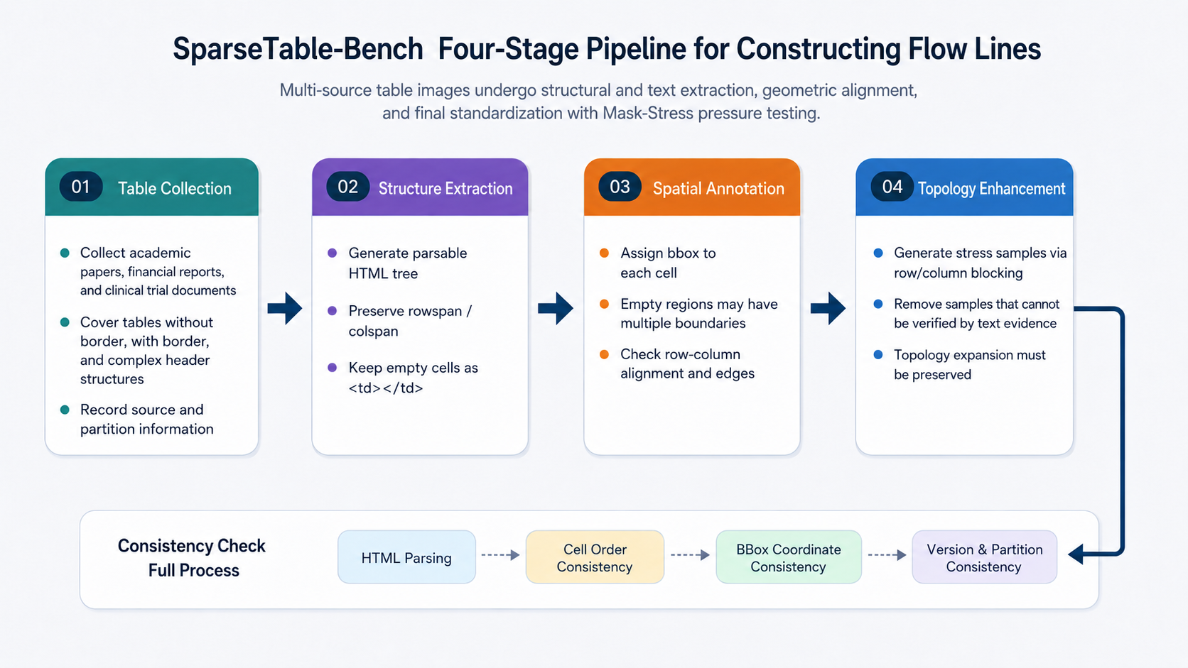
Figure 40-5: Four-stage SparseTable-Bench construction pipeline.

Case B.4.1 Table Collection¶

Raw table images are sourced from multi-source documents including scientific publications, financial reports, and clinical trial documents. These sources are chosen because they naturally contain large numbers of irregular tables: scientific papers frequently feature borderless experimental results tables and meta-analysis tables; financial reports commonly contain multi-level headers, blank groupings, and cross-column annotations; clinical trial documents routinely mix metrics, groups, time points, and missing observations within a single table. Compared with templated invoices or fixed-format forms, these tables are more likely to expose VLM dependencies on implicit structure.

The key at the collection stage is not to blindly increase the number of images, but to cover diversity in sparse structure. Data engineers must focus on at least four types of samples: tables lacking borders but with clearly aligned rows and columns; tables with large blank areas or many empty columns; tables containing complex rowspan/colspan relationships; and tables in which text density varies greatly across different regions. These samples constitute the foundation that distinguishes STB from ordinary dense-table datasets.

Case B.4.2 Structure Extraction¶

The structure extraction stage converts a table's logical topology into an HTML sequence. HTML is not the only viable format, but it offers two advantages: its tag tree naturally accommodates the hierarchical expression of rows, columns, and cells; and mainstream table structure metrics such as TEDS can be computed directly on HTML trees. For ordinary cells, annotations must specify the row and column to which each cell belongs; for merged cells, rowspan and colspan must be preserved; for empty cells, the corresponding <td> nodes must be retained rather than deleted due to the absence of text.

The most common error at this stage is "visually plausible but logically unparseable grids." For example, if a single empty <td> is missing from one row, a human reviewer may not notice, but after converting the HTML tree to a matrix, every subsequent column index in that row will be shifted left. Structure extraction therefore cannot rely solely on manual visual inspection; a parser should also be used to convert the HTML back into a grid matrix, checking the number of columns after each row is expanded, the coverage areas of merged cells, the count of empty positions, and the ordering of cells.

Case B.4.3 Spatial Annotation¶

The spatial annotation stage assigns two-dimensional bounding boxes to each cell. Bounding boxes are not merely auxiliary visualization fields; they determine whether the dataset can train and evaluate geometric alignment capability. For cells with text, the bounding box should cover the cell region rather than only the text region; for empty cells, bounding boxes must still be inferred from neighboring row-column boundaries, the overall table layout, and implicit grid structure. This allows the model to learn the structural prior that "a region without text may still be a valid cell."

Quality checks can be divided into geometric validity and topological consistency. Geometric validity covers coordinates within bounds, positive width and height, and bounding box dimensions consistent with image size. Topological consistency covers the requirement that cells in the same row have substantially overlapping vertical extents, cells in the same column have substantially aligned horizontal extents, and bounding boxes for merged cells cover the corresponding row-column areas. For sparse tables, topological consistency is often more important than text OCR, because large blank regions cannot be verified through text.

Case B.4.4 Sparse Topology Augmentation¶

The sparse topology augmentation stage is used to construct pressure tests and supplement robustness signals. Rather than simply randomly occluding the image, it applies controlled masking based on column, header, body, and cell topology. After occlusion, the corresponding regions in the image are filled with a uniform background color, and the text tokens in the annotations are simultaneously set to empty or removed, but the cell nodes, row-column positions, and topological relationships are preserved. Samples constructed this way reduce the model's reliance on local text cues, forcing it to use remaining layout, adjacent cells, and structural priors to recover the table.

The construction pipeline should ultimately produce three types of auditable artifacts: standard training/validation/test samples, STB-Mask-Stress pressure test samples, and data documentation recording the data version, source domains, split strategies, and transformation script hashes. Without this metadata, a benchmark easily becomes single-use experimental material, unable to support subsequent model iteration and cross-study comparison.

Case B.5: How Empty Cells and Sparse Layouts Induce Structural Errors¶

The core difficulty of sparse tables is not simply "too much whitespace, so too little information." Whitespace itself carries structural meaning. A blank region may represent an empty cell, an entire column of missing values, the area occupied by a spanning cell, or merely typographic whitespace on the page. If a model cannot distinguish among these cases, structural hallucinations will occur.

One typical error is empty-column skipping. Suppose a table truly has three columns, and the middle column is mostly empty. During generation, the model may output only the first and third columns, moving the content of the third column into the second-column position. At the text level, the major values have all been recognized; at the structural level, the column semantics have changed. In a financial statement, this may cause "current-period figures" to be interpreted as "prior-period figures"; in a clinical table, it may cause treatment-group metrics to be misassigned to the control group.

Another error is cascading misalignment. Table recognition typically generates output autoregressively; if a single empty <td> is missed earlier, all subsequent cells in that row shift left. If this error occurs in a multi-level header, the effect extends to multiple rows and multiple fields. Conventional average scores may show only a slight drop, but the actual business meaning has been completely distorted.

These structural errors are further reflected in evaluation results. In sparse tables, missing empty positions, column shifts, and erroneous filling of empty cells change the number of HTML nodes, node order, and row-column expansion relationships. They therefore usually reduce TEDS or TEDS-S. STB preserves HTML, text, and bounding boxes simultaneously so that score drops can be traced back to inspectable data objects rather than remaining only at the aggregate-metric level.

Errors in sparse tables can be classified into five types.

Table 40-7 summarizes the corresponding comparison and engineering considerations.

Table 40-7: Case B.5: How Empty Cells and Sparse Layouts Induce Structural Errors.

Error Type	Manifestation	Primary Cause	Observation Method in STB
Missing empty position	Empty `<td>` not generated; column count decreases	Empty cells lack visual text anchors	`[EMPTY_CELL]` recall, TEDS-S, row-column expansion check
Column left-shift / right-shift	Non-empty content placed in adjacent column	Intermediate empty column skipped or merged	HTML matrix alignment, bbox-to-column-index consistency
Empty-cell filling	Model generates nonexistent text in empty positions	Contextual completion or overly strong language prior	`[EMPTY_CELL]` precision, cell-text inspection
Incorrect merging relationships	`rowspan`/`colspan` missing or mislabeled	Sparse region boundaries are weak; header levels are complex	Structure tree edit, merge-area coverage check
Spatial drift	HTML structure parses correctly but bboxes do not align	Model learned sequences only, lacking geometric supervision	Cell bbox IoU, row-column geometric alignment check

These errors demonstrate that the value of SparseTable-Bench is not simply providing a more difficult dataset, but transforming structural failure modes in sparse tables into supervision objects that are annotatable, computable, and attributable.

Case B.6: STB-Mask-Stress: A Pressure Test for Information-Deficient Conditions¶

STB-Mask-Stress is the robustness evaluation split within SparseTable-Bench, dedicated specifically to pressure testing. Its design philosophy is to systematically reduce text cues — while preserving table topology — and to observe whether the model can still recover row-column structure and empty cell positions. Unlike ordinary data augmentation, the goal of STB-Mask-Stress is not to increase training set diversity, but to construct an evaluation environment that more closely resembles a "structural understanding stress test." This chapter follows the dataset documentation in using the name STB-Mask-Stress; in related experimental contexts, it can also be understood as a masked table evaluation setting oriented toward column-level occlusion, suitable for use with pressure-test metrics such as Masked-TEDS.

Figure 40-6 illustrates the basic workflow of STB-Mask-Stress, from column-level occlusion generation to evaluation interpretation.

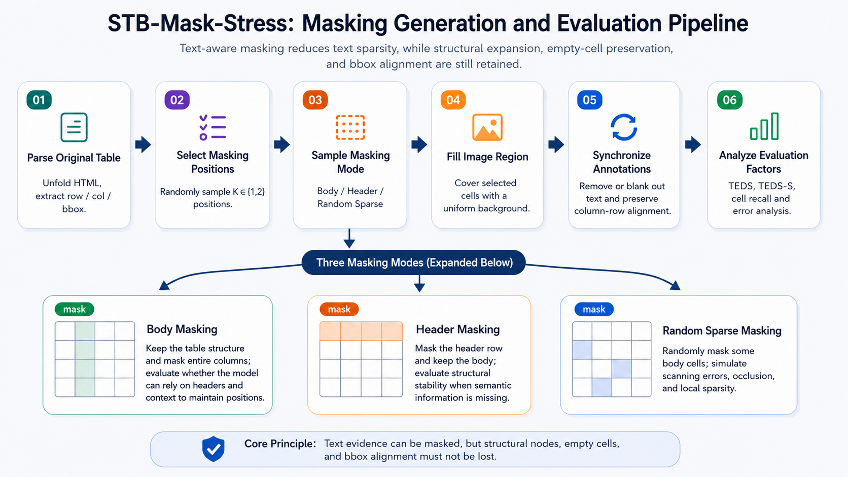
Figure 40-6: STB-Mask-Stress occlusion generation and evaluation workflow.

The occlusion strategy of STB-Mask-Stress is column-aware. The workflow can be summarized as follows.

Parse the original table structure to obtain the row-column index, header/body membership, and bounding box of each cell.
Randomly select a subset of columns as occlusion candidates.
Sample an occlusion pattern for each selected column. If the sampled probability falls in the body masking range, occlude the body cells in that column while preserving the header; if it falls in the header masking range, occlude the header cells while preserving the body; otherwise, randomly occlude a subset of body cells to produce intermittent blanks.
Fill the selected cell regions in the image with a uniform background color.
Synchronously update annotations: text tokens in occluded regions are removed from or set to empty in the target, but row-column topology is retained.
Compute TEDS, TEDS-S, or masked versions of structural metrics on the updated samples, and perform error attribution.

The three occlusion patterns assess different capabilities. Body Masking retains headers but removes body content, testing whether the model can maintain column positions based on column headers and geometric structure. Header Masking removes headers, testing whether the model can maintain body alignment when column semantics are absent. Random Sparse Masking produces local breaks and intermittent blanks, more closely approximating sparse conditions caused by real-world scanning artifacts, occlusions, or rendering defects.

It must be emphasized that STB-Mask-Stress scores should not be equated directly with standard test set generalization scores. The standard test set measures the model's overall recognition ability on natural tables; the pressure test measures the model's structural recovery ability under information-deficient and visually sparse conditions. A model with a high TEDS on the standard test but a noticeably lower TEDS-S on STB-Mask-Stress likely depends on visible text anchors rather than having stably learned row-column topology. Conversely, a model with a stable structural score on the pressure test but a dropping text score may have preserved the topology while being unable to recover occluded content — this represents a different type of capability boundary.

From a data engineering perspective, the key to pressure testing is "occlusion and annotation synchronization." If images are occluded without updating labels, the model is required to predict invisible text, and evaluation results will conflate language memorization and guessing ability. If text is removed while also deleting cell nodes, the pressure test degenerates into an ordinary sparse table, making it impossible to test empty-position preservation. STB-Mask-Stress should therefore always uphold one principle: text evidence may be removed; structural topology must not be arbitrarily eliminated.

Case B.7: Evaluation Protocol: TEDS, TEDS-S, and Error Interpretation¶

SparseTable-Bench uses Tree-Edit-Distance-based Similarity (TEDS) and its structural variant TEDS-S as primary evaluation metrics. TEDS parses both the predicted HTML and the reference HTML into trees, computing a normalized tree-edit similarity. It is jointly influenced by structural tags, node ordering, and cell text content. TEDS-S ignores text content and focuses more on structural topology — for example, row-column alignment, merged cell recovery, and empty cell positions.

These two metrics are appropriate for cross-model comparison, but must not be interpreted mechanically. Especially for sparse table datasets such as STB, metric differences often correspond to different error sources.

In extremely sparse tables or tables with many empty cells, lower TEDS/TEDS-S scores usually originate from structural prediction errors. Numerous empty positions weaken visible text anchors. A model may fill nonexistent content into empty cells, skip empty columns, or assign neighboring-column content to the wrong column position. Once these errors enter the HTML output, the number of <td> nodes, node order, and row-column expansion relationships change, ultimately reducing TEDS or TEDS-S. TEDS-S further focuses on structural topology and empty-cell positions, making it especially useful for exposing such row-column alignment errors.

Table 40-8 summarizes the corresponding comparison and engineering considerations.

Table 40-8: Case B.7: Evaluation Protocol: TEDS, TEDS-S, and Error Interpretation.

Metric Pattern	Possible Interpretation	Conclusion That Should Not Be Drawn	Supplementary Check
TEDS high, TEDS-S high	Structure and text are broadly stable	Does not imply bboxes are necessarily correct	Cell bbox IoU, row-column geometric alignment
TEDS low, TEDS-S high	Structure is largely correct but text content is wrong	Does not imply the model has poor structure recognition	OCR/text normalization, number formatting
TEDS-S low, TEDS close or slightly higher	Some text is correct but structural misalignment exists	Cannot rely on text match rate alone	Empty-cell recall, column-shift inspection
Standard set high, Mask-Stress low	Depends on visible text anchors; poor resistance to sparseness	Does not imply the model is unusable in ordinary scenarios	Statistics broken down by occlusion pattern: body/header/random
Mask-Stress TEDS-S high but TEDS low	Topology well preserved, occluded text unrecoverable	Cannot require the model to recover invisible content from nothing	Confirm that occluded text has been synchronously removed from targets

When interpreting TEDS/TEDS-S in STB, three types of information should be considered together.

First, TEDS is a mixed metric of structure and text. It is appropriate for assessing how closely the final HTML output approximates the reference, but when scores drop, it is necessary to disaggregate the causes — text misrecognition, tag-tree errors, or cell ordering misalignment. For sparse tables, the same TEDS decrease may represent entirely different risks.

Second, TEDS-S is a structural metric, but not a geometric metric. By ignoring text, it more clearly reflects row-column topology, but it is still tree-based and does not directly verify whether bounding boxes correspond to image positions. If a model outputs a topologically correct HTML structure but places cell bounding boxes in incorrect visual regions, TEDS-S will not adequately penalize this. For geometrically aware models using STB, additional checks such as bbox IoU, centroid distance, row-column alignment error, or cell-to-region assignment should be added.

Third, pressure test scores should be reported by occlusion type. Body Masking, Header Masking, and Random Sparse Masking assess different capabilities. Reporting only a single average score may conceal differences such as the model collapsing when headers are absent, remaining stable under body occlusion, and drifting under random sparseness. Data engineering practice typically reports the overall score together with per-mask-type scores and representative failure cases.

In addition to the primary metrics, STB is well suited to introducing several diagnostic metrics. For example, empty-cell recall measures whether [EMPTY_CELL] positions are preserved; column-count expansion consistency measures whether each row, when expanded, matches the reference column count; merged-cell accuracy measures rowspan/colspan correctness; and bbox match rate measures whether structural nodes correspond to their visual regions. These metrics need not all appear in leaderboards, but they are highly suited for model debugging and data quality inspection.

Case B.8: Data Engineering Practice: Using STB for Training and Reproduction¶

When using SparseTable-Bench for model training, the most common approach is to use images as input and organize HTML structure, cell text, and bounding boxes into a unified output sequence or multi-task supervision target. For generative VLMs, the model can directly generate HTML and insert text or empty-cell tokens at the cell content positions; for models with position heads, bbox regression or coordinate token prediction can be added alongside text generation; for adapter-based or structural prior models, bounding boxes and grid topology can be converted into auxiliary structural features to help the decoder maintain row-column alignment during generation.

Several constraints are easily overlooked in practice.

First, data transformation must maintain consistent sample ordering. The i-th cell in the HTML, cells[i].text, and cells[i].bbox must refer to the same logical cell. If a transformation script alters the ordering while filtering empty text, expanding merged cells, or sorting bounding boxes, the training target becomes noise.

Second, empty cells must not be deleted during the cleaning stage. Many general-purpose document cleaning scripts filter out empty strings, empty tags, and empty bounding boxes as invalid fields. In STB, these are precisely the core supervision signals that must be preserved. Cleaning rules must therefore distinguish between "invalid missing data" and "valid empty cells."

Third, bounding box coordinates require an explicit coordinate system. Different models may use original pixel coordinates, normalized coordinates, or discrete token coordinates. Transformations should record image width and height, scale factors, and padding strategies to prevent training and evaluation from using different coordinate systems.

Fourth, standard test results and pressure test results must be reported separately. If STB-Mask-Stress is mixed into a general test set average, reviewers will have difficulty determining whether the model's shortfall reflects insufficient generalization on natural scenarios or insufficient robustness in extremely sparse scenarios. A clearer reporting format is: first present TEDS/TEDS-S on the Standard Test, then present TEDS/TEDS-S on the Mask-Stress split, broken down by occlusion type.

Fifth, error cases should be traced back to data objects. A single failure can be decomposed into several questions: Is the HTML parseable? Is the row-column expansion consistent? Were any empty cells missed? Was any text misread? Were any bounding boxes offset? Only by doing so do model fix actions become concrete: whether more empty-cell samples are needed, position supervision needs improvement, the tokenizer needs correction, or annotations need re-validation.

For reproducibility, using STB should not stop at the coarse-grained procedure of "load data, train model, report score." A more rigorous approach is to decompose each experiment into four auditable stages. Stage one is data loading verification: randomly sample training, validation, standard test, and pressure test samples to confirm that the image, HTML, cell list, and bounding boxes can all be associated through a single sample ID. Stage two is schema rendering verification: expand the HTML into a two-dimensional grid and overlay bounding boxes on the original image to confirm that empty cells, merged cells, and non-empty text are visually interpretable. Stage three is model input-output verification: clarify whether the model receives the original image, a cropped image, or a patch-based image, and whether it outputs pure HTML, HTML with coordinate tokens, or multi-task HTML and bbox results. Stage four is evaluation and attribution verification: compute Standard-Test and STB-Mask-Stress scores separately, then sample and review failures by the four error categories of empty-position miss, column shift, text error, and spatial drift.

Table 40-9 summarizes the corresponding comparison and engineering considerations.

Table 40-9: Case B.8: Data Engineering Practice: Using STB for Training and Reproduction.

Reproduction Stage	Input Objects	Output Objects	Key Checks
Data loading	Image, HTML, cells, bbox	Unified sample record	ID alignment, field completeness, correct split assignment
Schema rendering	HTML tree, cell list	Two-dimensional grid and visualization overlay	Empty cells preserved, merge relationships parseable, bboxes within bounds
Model training	Table images and multi-task labels	HTML sequence, text tokens, bbox predictions	`[EMPTY_CELL]` vocabulary consistency, coordinate system consistency, reasonable loss masking
Evaluation attribution	Predicted results and reference annotations	TEDS, TEDS-S, diagnostic error table	Standard set and pressure set reported separately; errors traceable to data fields

For VLM or document model training, STB can serve two different roles. As training data, it provides structured visual supervision suited to helping models learn the alignment from "visual regions to logical cells." As evaluation data, it is better positioned as a robustness slice for verifying whether models depend solely on text density and local OCR cues. If a general-purpose VLM performs well on natural image QA but cannot preserve empty columns on STB-Mask-Stress, its document structural capability still requires specialized data reinforcement. If a document model has high structural scores on the standard test but exhibits extensive spatial drift in bbox verification, the model may have learned HTML language patterns without having genuinely established geometric alignment ability.

Therefore, in coursework experiments or project work, STB evaluation results are typically decomposed into two layers: "usability" and "robustness." The usability layer examines table structure recovery quality on the standard test set, answering whether the model can handle typical scientific, financial, and clinical tables. The robustness layer examines empty cells, occluded columns, and locally sparse regions in the pressure test, answering whether the model can maintain a credible structure when evidence is absent. This layered reporting approach is more suitable for data engineering retrospectives than a single leaderboard score, and more readily supports the flow of failure samples back into cleaning, annotation, and retraining pipelines.

In team collaboration, STB should also be elevated from "experimental data" to "deliverable data asset." A deliverable version should include at minimum three types of records. The first type is a data card recording data provenance, license status, sample size, split methodology, field schema, empty-cell conventions, and the bounding box coordinate system. The second type is an evaluation card recording the model used, input resolution, decoding parameters, TEDS/TEDS-S computation script version, whether OCR post-processing is enabled, and the occlusion strategy for Mask-Stress. The third type is an error card recording representative failure samples, error types, whether caused by annotation issues, whether caused by model output issues, and the next round of corrective actions. Without these records, even if scores are reproducible, the causes of failures are difficult to audit.

In particular, errors related to empty cells should not appear only as a few case screenshots in the final report. A better practice is to consolidate them into queryable error slices — for example, "entire column empty but column header visible," "column header empty but body dense," "blank region spanning multiple rows," and "empty cell adjacent to merged cell." Each slice can independently report TEDS-S, empty-cell recall rate, and column-expansion consistency rate. This way, when a new model version improves on the average score but regresses on the empty-column slice, the data team can promptly detect the robustness regression rather than waiting until incorrect column interpretation surfaces on the business side.

Annotation quality inspection can also adopt a dual-channel approach. The first channel checks structure: whether the HTML can be stably parsed into a two-dimensional matrix, whether the row and column counts are consistent after expansion, and whether rowspan and colspan produce overlaps or holes. The second channel checks geometry: whether bounding boxes are within bounds, whether they cover the cell region, whether the horizontal extents of cells in the same column are continuous, and whether bounding boxes for empty cells together with adjacent cells form a reasonable grid. Only when both structure and geometry pass should a sample enter the training set; if text is correct but structure or bounding boxes are suspect, the sample should enter a rework queue rather than be used directly as a supervision signal.

A reproducible benchmark version requires pinned version numbers for the training set, validation set, standard test set, and STB-Mask-Stress, along with retained hash values of data generation scripts. Pressure tests especially require versioning, because small changes to the number of occluded columns, occlusion probability, or background fill value all affect model scores. If the occlusion strategy is adjusted in the future, it should be released as a new pressure test version rather than overwriting existing results. Only then can STB support long-term model iteration, cross-team comparison, and in-book project reproducibility experiments.

Case B.9: MindSpore Implementation and Code¶

To facilitate experimental reproduction and review of data processing workflows, the MindSpore companion implementation entry point for SparseTable-Bench is:

champiom666/SparseTable-Bench-MindSpore

This repository serves as the companion implementation entry for this chapter, organizing data reading, occlusion construction, and evaluation reproduction experiments. A complete companion implementation should typically include: an STB data reader; HTML and cell schema transformation scripts; [EMPTY_CELL] token normalization; bounding box coordinate transformation; an STB-Mask-Stress generation script; TEDS/TEDS-S evaluation scripts; and a minimal example configuration for MindSpore training. Only then can a closed loop be formed among the book chapter, dataset documentation, and code repository.

In addition to the GitHub code entry, the public dataset address should cross-reference the code repository in the README:

https://huggingface.co/datasets/champion666/SparseTable_Bench_Dataset

The role of the code repository is not to simply replicate paper experiments, but to support reproduction of the data engineering workflow described in this chapter: loading samples, validating the schema, constructing occlusions, running evaluation, and interpreting errors. As long as these interfaces remain stable, subsequent substitution of SA-Table, OCRFlux, Qwen-VL, or any other table recognition model can be compared under the same data protocol.

Case B.10: Connections to Adjacent Chapters¶

SparseTable-Bench connects naturally to multiple parts of this book.

With respect to the document understanding and cross-modal alignment topics in Part 3, STB provides a stricter example than ordinary OCR: visual regions, text content, and structure tokens must be simultaneously aligned. The OCR and document structure re-annotation discussed in Chapter 9 is concretely instantiated here as the synchronization of cell-level text, bounding boxes, and HTML. The cross-modal alignment discussed in Chapter 11 is concretely instantiated here as the alignment of table image regions with logical cell nodes. This chapter can therefore be viewed as a specialized case study advancing from "page text recognition" toward "structured visual object recovery."

Compared with Chapter 40 on invoice document understanding, StructBill-CN places greater emphasis on business schemas, field extraction, and logical consistency, while SparseTable-Bench places greater emphasis on intra-table topology, empty cells, and sparse layouts. Both belong to visual document data engineering, but one targets high-risk invoice fields and the other targets general table structure robustness.

Compared with Chapter 41 on multi-chart infographic reasoning, STB focuses on structural recovery within a single table object, while multi-chart infographic reasoning focuses on cross-chart evidence aggregation and multi-step computation. The former provides foundational capability for the latter: if a model cannot stably recover column positions within a single table, numerical reading and evidence localization in cross-chart reasoning will lose their reliable basis.

Looking ahead, STB connects directly to Chapter 47 on VLM data recipes. Chapter 47 examines how multimodal training data organizes images, text, coordinates, and instruction signals; STB provides exactly such a structured visual supervision example: the input is a table image, and the output simultaneously includes HTML structure, cell text, bounding boxes, and empty-cell placeholders. It can serve as a document-table slice in VLM data recipes, demonstrating why general image-caption pairs are insufficient for training stable table structure capability.

In the Part 14 projects, STB can also connect to P03 and P05. The LLaVA multimodal instruction data factory in P03 needs to convert document images into trainable visual instruction samples; STB can provide instruction sources such as "identify the table structure," "indicate the positions of empty cells," and "explain column-position shift errors." The multimodal RAG project in P05 needs to extract retrievable evidence from PDFs, financial reports, and scientific publications; STB can help parse tables into structured evidence that is citable, comparable, and traceable. Particularly in financial reports, medical papers, and scientific publications, table structure errors are often harder to detect and more likely to affect final answers than individual OCR character errors.

Case B: Summary¶

The core contribution of SparseTable-Bench is that it transforms the problem of structural robustness in sparse tables into a data engineering problem that is annotatable, trainable, and evaluable. The dataset establishes three categories of supervision signals through HTML structure sequences, cell-level text content, and fine-grained bounding boxes, and uses [EMPTY_CELL] to explicitly preserve empty-cell topology, preventing blank regions from being incorrectly removed during cleaning, training, and evaluation. STB-Mask-Stress further constructs pressure tests through column-aware occlusion, enabling the model's structural recovery capability under severe information deficiency to be observed in isolation.

When using this dataset, relying on a single overall TEDS score is insufficient. TEDS, TEDS-S, bounding box inspection, empty-cell recall, and per-mask-type error analysis should be used in combination to distinguish text errors, structural errors, and spatial errors. The value of STB is not simply providing a "harder" table dataset, but transforming the failure patterns of sparse tables into objects that are annotatable, trainable, and evaluable. For large model data engineering, the lesson of STB is this: the value of a complex document dataset comes not only from sample scale, but from whether real failure patterns have been encoded into the schema, the construction workflow, and the evaluation protocol.

Chapter Summary¶

This chapter examined invoice and bill understanding together with sparse-table structure recovery as two branches of visual document data engineering. The former emphasizes business fields, layout evidence, and logical consistency; the latter emphasizes table topology, empty cells, occlusion robustness, and structural evaluation. Together they show that visual document datasets cannot remain at the level of image-text pairs or OCR text alone. They must encode field schemas, spatial grounding, structural constraints, failure modes, and quality audit mechanisms as part of the data design.

For subsequent multimodal model training, the core lesson is that the publication-grade and production-grade value of document data depends on whether the data can reliably express traceable relationships among image regions, textual content, structural objects, and business semantics. Only when these relationships are encoded clearly can the dataset support reproducible training, interpretable evaluation, and continuous improvement in real application settings.

References¶

Bai S, Chen K, Liu X, et al. (2025) Qwen2.5-VL Technical Report. arXiv preprint arXiv:2502.13923.

Blecher L, Cucurull G, Scialom T, Stojnic R (2023) Nougat: Neural Optical Understanding for Academic Documents. arXiv preprint arXiv:2308.13418.

Huang Y, Lv T, Cui L, Lu Y, Wei F (2022) LayoutLMv3: Pre-training for Document AI with Unified Text and Image Masking. Proc. ACM Multimedia.

Huang Z, Chen K, He J, Bai X, Karatzas D, Lu S, Jawahar CV (2019) ICDAR2019 Competition on Scanned Receipt OCR and Information Extraction. Proc. ICDAR, pp. 1516-1520.

Hu EJ, Shen Y, Wallis P, Allen-Zhu Z, Li Y, Wang S, Wang L, Chen W (2021) LoRA: Low-Rank Adaptation of Large Language Models. arXiv preprint arXiv:2106.09685.

Jaume G, Ekenel HK, Thiran J-P (2019) FUNSD: A Dataset for Form Understanding in Noisy Scanned Documents. ICDAR Workshop.

Kuhn HW (1955) The Hungarian Method for the Assignment Problem. Naval Research Logistics Quarterly, 2(1-2), pp. 83-97. https://doi.org/10.1002/nav.3800020109.

Levenshtein VI (1965) Binary Codes Capable of Correcting Deletions, Insertions and Reversals. Soviet Physics Doklady, 10, pp. 707-710.

Liu H, Xue W, Chen Y, et al. (2024) A Survey on Hallucination in Large Vision-Language Models. arXiv preprint arXiv:2402.00253.

Mathew M, Karatzas D, Jawahar CV (2021) DocVQA: A Dataset for VQA on Document Images. Proc. WACV. https://doi.org/10.1109/wacv48630.2021.00225.

Niu J, Liu Z, Gu Z, et al. (2025) MinerU 2.5: A Decoupled Vision-Language Model for Efficient High-Resolution Document Parsing. arXiv preprint.

Park S, Shin S, Lee B, et al. (2019) CORD: A Consolidated Receipt Dataset for Post-OCR Parsing. NeurIPS Workshop on Document Intelligence.

Rafailov R, Sharma A, Mitchell E, Ermon S, Manning CD, Finn C (2024) Direct Preference Optimization: Your Language Model Is Secretly a Reward Model. Proc. NeurIPS. arXiv:2305.18290.

Schulman J, Wolski F, Dhariwal P, Radford A, Klimov O (2017) Proximal Policy Optimization Algorithms. arXiv preprint arXiv:1707.06347.

Shao Z, Wang P, et al. (2024) DeepSeekMath: Pushing the Limits of Mathematical Reasoning in Open Language Models. arXiv preprint arXiv:2402.03300.

Tianchi A, CHIP Committee (2022) CHIP 2022 Shared Task: Medical Invoice OCR Element Extraction Dataset. Aliyun Tianchi Platform.

Xu Y, Li M, Cui L, Huang S, Wei F, Zhou M (2020) LayoutLM: Pre-training of Text and Layout for Document Image Understanding. Proc. ACM SIGKDD, pp. 1192-1200.

Xue W, Yu B, Wang W, Tao D, Li Q (2021) TGRNet: A Table Graph Reconstruction Network for Table Structure Recognition. arXiv preprint arXiv:2106.10598.

Yang Z, Long R, Wang P, et al. (2023) Modeling Entities as Semantic Points for Visual Information Extraction in the Wild. Proc. CVPR.

Zhang N, Chen M, Bi Z, et al. (2022) CBLUE: A Chinese Biomedical Language Understanding Evaluation Benchmark. Proc. ACL, pp. 7888-7915. https://doi.org/10.18653/v1/2022.acl-long.544.

Zhong X, ShafieiBavani E, Jimeno Yepes A (2020) Image-based Table Recognition: Data, Model, and Evaluation. arXiv preprint arXiv:1911.10683.

Bai S, Cai Y, Chen R, et al. (2025a) Qwen3-VL Technical Report. arXiv preprint.

ChatDOC (2025). OCRFlux-3B: A Multimodal Large Language Model for Document Parsing. Hugging Face Model Card.

Cui C, Sun T, Liang S, et al. (2025) PaddleOCR-VL: Boosting Multilingual Document Parsing via a 0.9B Ultra-Compact Vision-Language Model. arXiv preprint.

Guo D, Yang D, Zhang H, et al. (2025) DeepSeek-R1: Incentivizing Reasoning Capability in LLMs via Reinforcement Learning. arXiv preprint arXiv:2501.12948.

Hunyuan Vision Team (2025). HunyuanOCR Technical Report. arXiv preprint.

Li Y, Yang G, Liu H, Wang B, Zhang C (2025a) Dots.OCR: Multilingual Document Layout Parsing in a Single Vision-Language Model. arXiv preprint.

Poznanski J, Soldaini L, Lo K (2025) olmOCR 2: Unit Test Rewards for Document OCR. arXiv preprint arXiv:2510.19817.

Smock B, Faucon-Morin V, Sokolov M, et al. (2025) PubTables-v2: A New Large-Scale Dataset for Full-Page and Multi-Page Table Extraction. arXiv preprint arXiv:2512.10888.

Wang W, Gao Z, Gu L, et al. (2025) InternVL3.5: Advancing Open-Source Multimodal Models in Versatility, Reasoning, and Efficiency. arXiv preprint arXiv:2508.18265.

Zhang J, Liu Y, Wu Z, et al. (2025) MonkeyOCR v1.5 Technical Report: Unlocking Robust Document Parsing for Complex Patterns. arXiv preprint.

Smock B, Pesala R, Abraham R (2022) PubTables-1M: Towards Comprehensive Table Extraction From Unstructured Documents. Proc. CVPR. https://doi.org/10.1109/cvpr52688.2022.00459.

Zhu F, Lei W, Huang Y, Wang C, Zhang S, Lv J, Feng F, Chua T-S (2021) TAT-QA: A Question Answering Benchmark on a Hybrid of Tabular and Textual Content in Finance. Proc. ACL. https://doi.org/10.18653/v1/2021.acl-long.254.

Pandas Development Team (2026) pandas Documentation. https://pandas.pydata.org/docs/.

Apache Arrow Contributors (2026) Apache Arrow Documentation. https://arrow.apache.org/docs/.